Introduction to Google Earth Engine
Estéban Hamel & Arthur de Granpré
January 2021
- Summary
- Objectives
- Step 1: Interface overview
- Step 2: Select a region of interest with geometry tools
- Step 3: Load and display elevation layer
- Step 4 Work with satellite imagery for a region of interest
- Step 5: Display a satellite image with the boundaries of a shapefile
- Step 6: Calculate a spectral index (ex: NDVI)
- Step 7: Image classification with Google Earth Engine
- Step 8: Export raster layer to Google Drive
- Step 9: Draw graph with GEE
Summary
This workshop is an introduction to Google Earth Engine (GEE).
Earth Engine is online software from Google that allows users to manipulate and analyze lots of geographical layers (satellite imagery, climate data, topographic layers, etc.). An advantage of using GEE is that most of the calculations are done online on Google cloud and not on a personal computer. The following manipulations are an introduction to GEE tools with coding chunks that are easy to reproduce and adapt to users needs.
Objectives
- Import and visualize satellite images from a region of interest for a given moment;
- Work with satellites images delimited by a shapefile;
- Calculate an NDVI layer from a satellite image;
- Make an image classification;
- Export layer from GEE in a raster format;
- Make graphs with GEE.
Step 1: Interface overview
First, you need to have a Google account to access the GEE plateform.
You can sign up to GEE with your Gmail identifiant to the following link: https://signup.earthengine.google.com/#!/.
Once you register to GEE, you can access the code editor to this link: https://code.earthengine.google.com/.
Here’s some information about the interface.
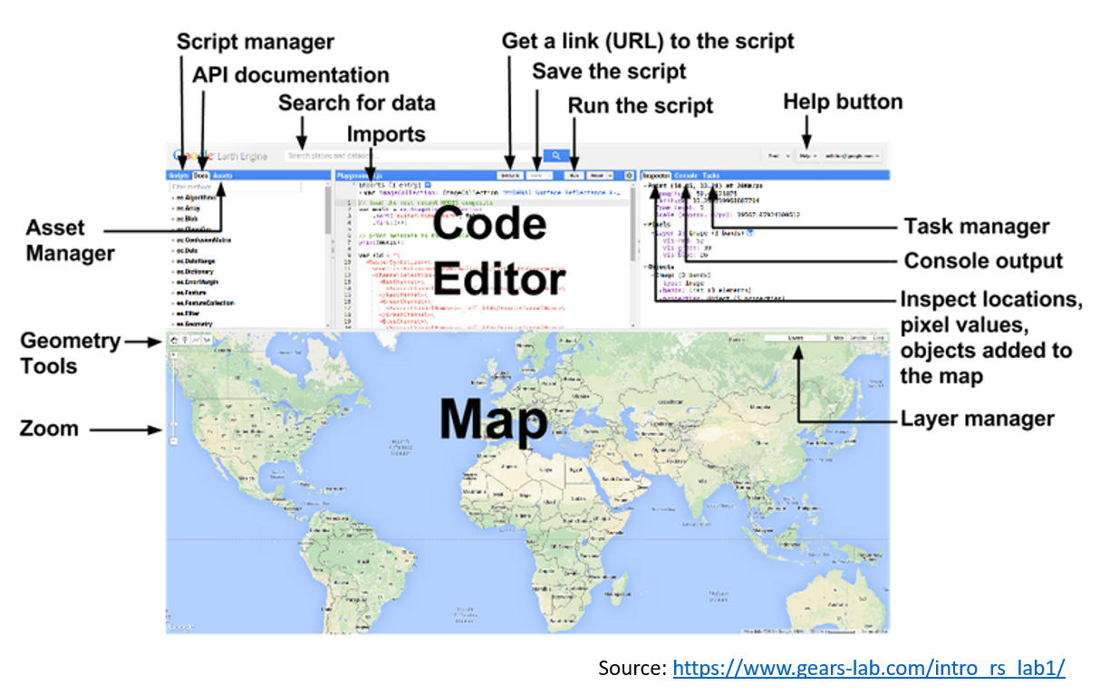
Left Panel
- Scripts tab for managing your programming scripts.
- Docs tab for accessing documentation of Earth Engine objects and methods, as well as a few that are specific to the Code Editor application.
- Assets tab for managing assets that you upload.
Center Panel
- Code editor where you write and edit code
Right Pannel
- Console tab for printing output.
- Inspector tab for querying map results.
- Tasks tab for managing long running tasks.
Search Bar
- For finding datasets and places of interest
Map
- Interactive map where the calculated layers are shown over a typical Google map interface.
Step 2: Select a region of interest with geometry tools
Start by navigating to La Mauricie National Park. You can search “Shawinigan” in the search bar to help you to locate the place.
- With the geometry tool, add a landmark by clicking on the landmark pictogram and put a point in the middle of the National Park.
- Click on “Exit” once the landmark is in place to avoid adding other points.
- Rename the landmark “pnm” in the script.
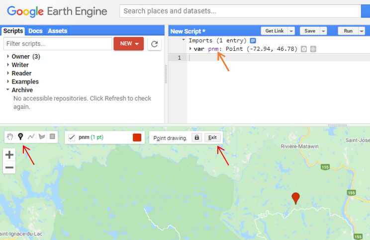
An alternative to geometry tools is to type this code to place a landmark. To complete the landmark you would have to click on the import option given by the code after typing it.
var pnm = /* color: #d63000 */ee.Geometry.Point([-72.97, 46.74])
Do not forget to save you script with the Save button.
Step 3: Load and display elevation layer
To import a dataset, you have to import it from Earth Engine database. To do so, you can use the search bar to search for the dataset needed. Once it is imported, the dataset will not be displayed automatically. You will have to define visualization parameters and boundaries around where you want to display the dataset, otherwise it will display the dataset for all its entire area.
- To add elevation layer, search and import NASA SRTM Digital Elevation 30m in the search bar.
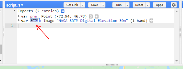
- You can read the available information about this dataset by clicking on the search result and look at the different tabs. You can press “import” to load the layer in you script.
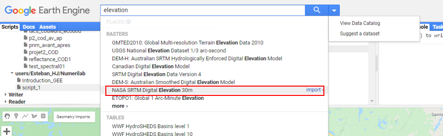
- You can rename the layer “srtm”.
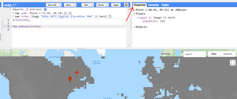
- Use the following code to print the information about the layer in the console.
// Print information from the dataset in the right console
print(srtm);
- To display “srtm” layer, use the tool Map.addLayer.
// Display the elevation layer
Map.addLayer(srtm);
- The layer is not really precise for the region of interest because you did not define any visualization parameters. Try the following command that gives a range of values for the layer, and also a name.
// Give a range of value to display the elevation layer
Map.addLayer(srtm, {min: 0, max: 400},"Elevation");
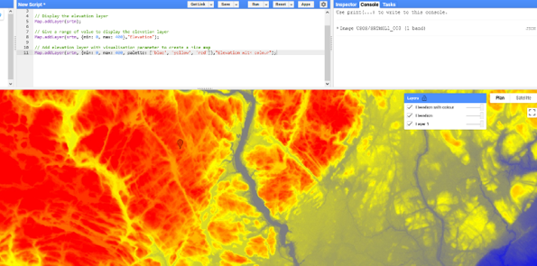
- You could also add a colour gradient to the layer to create a better map.
// Add elevation layer with visualisation parameter to create a nice map
Map.addLayer(srtm, {min: 0, max: 400, palette: ['blue', 'yellow', 'red']},"Elevation with colour");
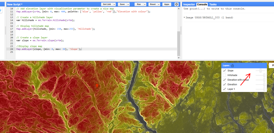
- Elevation data is useful, but others tools can complement it like hillshade and slope of an area. The tools ee.Terrain.hillshade() and ee.Terrain.slope() can rapidly display this information.
// Create a hillshade layer
var hillshade = ee.Terrain.hillshade(srtm);

// Display hillshade map
Map.addLayer(hillshade, {min: 150, max:255}, 'Hillshade');
// Create a slope layer
var slope = ee.Terrain.slope(srtm);

//Display slope map
Map.addLayer(slope, {min: 0, max: 30}, 'Slope');
Step 4 Work with satellite imagery for a region of interest
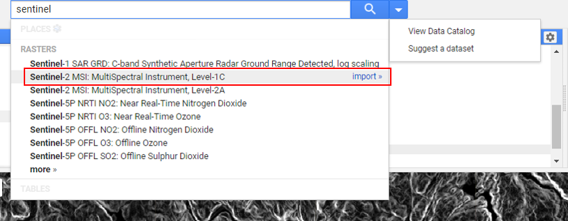
Google Earth Engine dataset allows us to work with tons of satellite images. To focus on a region of interest you will have to apply some filters. Begin by importing images from Sentinel 2 satellite. It would be also possible to work with Landsat images.
- Start by searching for “sentinel” in the search bar and select “Sentinel-2 MSI: Multispectral Instrument, Level-1c. Import this layer and rename it “sent2”.
-The following lines define some filters for the region of interest selected earlier in La Mauricie National Park: between September and October 2020, and for the least cloudy image possible. You can also print the result of your query in the console with the function .size to get an idea of the number of images available depending on your filter.
// Create a variable for the satellite image
var pnm_s2=sent2
    .filterBounds(pnm) // Geographical filter
    .filterDate("2020-07-01", "2020-08-30") // Temporal filter
    .filterMetadata('CLOUDY_PIXEL_PERCENTAGE','less_than',10);// Filter for image clearness

// Query for number of picture corresponding to all filters
print(pnm_s2.size(),"n. images");
The previous code allows us to display many images at the same time. The next one will be preferencially select the best images according to filter applied.
// Create an object that contain the satellite image selected
var pnm_i = sent2
    .filterBounds(pnm) // Geographical filter
    .filterDate("2020-07-01", "2020-09-30") // Temporal filter
    .sort("CLOUD_COVERAGE_ASSESSMENT") // Filter for image clearness
    .first(); // Select the less cloudy image

print(pnm_i,"Best image");
//extra : 2nd best?
var pnm_i2 = sent2
    .filterDate("2020-07-01", "2020-09-30")
    .filterBounds(pnm)
    .sort("CLOUD_COVERAGE_ASSESSMENT")
    .select(1);  //first index is 0, so the 2nd best image will be selected by 1
print(pnm_i2, "2nd best image");
- In order to display the image created previously, use the Map.addLayer tool and define visualization parameters for the red, blue and green bands.
// Define visualization parameters
var rgb_colour = {
        bands: ["B4", "B3", "B2"],
        min: 0,
        max: 1850
        };

Map.addLayer(pnm_i,rgb_colour,"Sentinel-2 Image");
Step 5: Display a satellite image with the boundaries of a shapefile
In the previous step you worked with the landmark placed in La Mauricie National Park. It would be also possible to import a shapefile in order to work within a specific area. In this step you will have to import a shapefile and associate it to the National Park in order to display an image exclusively in this area.
- First go in the assets tabs –> New –> Shapefiles
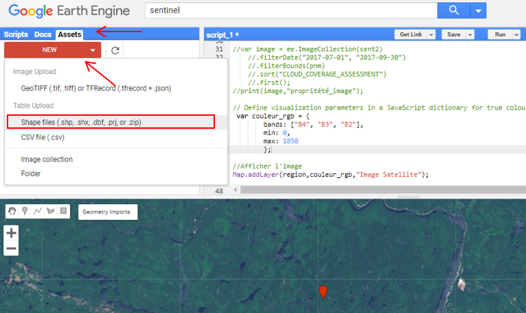
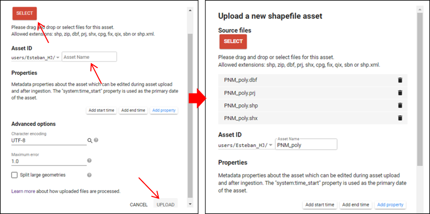
- Select the files that end with .shp; .dbf; .shx; .prj associated to the desire shapefile from the folder located on your computer. –> Type the name that you want to give to the shapefile ex. “PNM_poly”. –> Upload
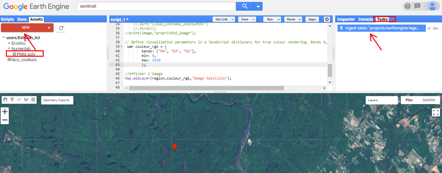
- To validate the importation, take a look at the task manager in the right panel. Once the file is uploaded, the download bar should be full. When you update the asset tab, you should see your shapefile layer imported in the assets tabs in the left panel.
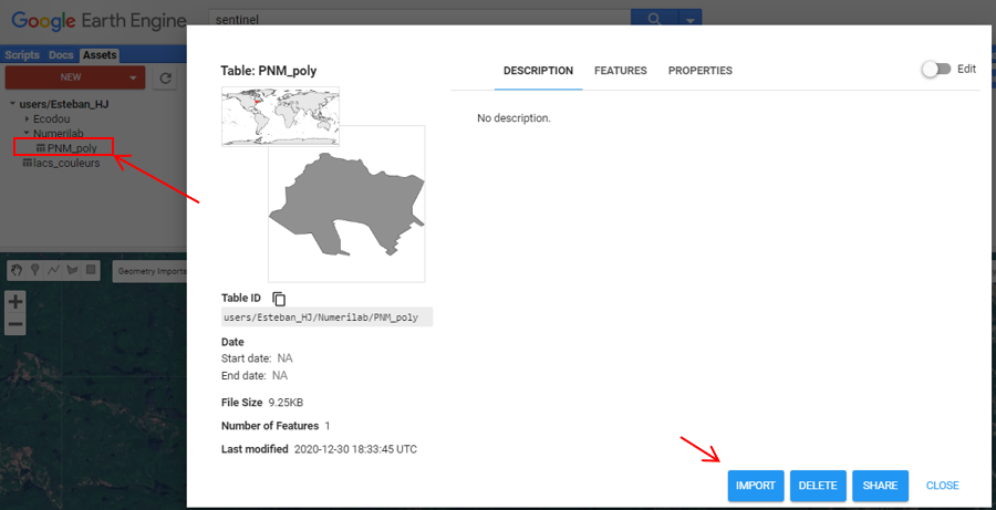
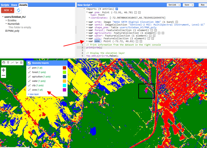
- To import the shapefile layer in your script you can click on the desired layer at the assets tab. –> Import –> Rename the layer “shape_pnm” in the script.
- This line could have worked too. It defines a variable from your shapefile layer.
// Add a variable corresponding to a shapefile
var pnm_poly = ee.FeatureCollection('users/XXX/PNM_poly');
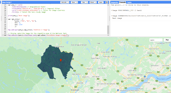
- When the shapefile is imported, it is easy to display the satellite image for the shapefile area with the clip tool.
// Display satellite image for the shapefile area of the National Park
Map.addLayer(pnm_i.clip(shape_pnm),rgb_colour,"Satellite Image cropped");
Step 6: Calculate a spectral index (ex: NDVI)
Another exercise with Google Earth Engine is to create a new layer which contains a calculated band like NDVI index (Normalized Difference Vegetation Index).
This type of index is often used to highlight some element of an existing image. In the case of NDVI, it is a ratio between reflectance of red and near infrared bands that highlight the presence of vegetation in an image. The formula to calculate NDVI is shown here.
\(NDVI = \frac{NIR-RED}{NIR+RED}\)
- There is different method to calculate this kind of layer.
- By using a function.
// Creating the function
var ndvi = function (x) {
  var result=x.normalizedDifference(["B8", "B4"]).rename("NDVI");
  return x.addBands(result);
};

// Apply the function to an image
var ndvi1 = ndvi(pnm_i);

// Display the result
Map.addLayer(ndvi1, {bands:['NDVI'],min:0,max:1,palette:['red','yellow','green']},"NDVI Method1");
- By using an expression that calculate difference between bands.
// Create the expression to calculate
var ndvi2 = pnm_i.expression(
     "(NIR - RED) / (NIR + RED)",
    {
      RED: pnm_i.select("B4"),
      NIR: pnm_i.select("B8"),
 }).rename('NDVI'); // Give a name to the band you created

// Display the result
Map.addLayer(ndvi2, {min: 0, max: 1,palette:['cyan','green','orange'] }, "NDVI Method 2");
Step 7: Image classification with Google Earth Engine
This exercise is about image classification with GEE. The following code makes a supervised classification of an image for different type of landscape. First, you need to build a training dataset where landscapes are known. After you can reuse the training data to extend the analysis to a bigger scale.
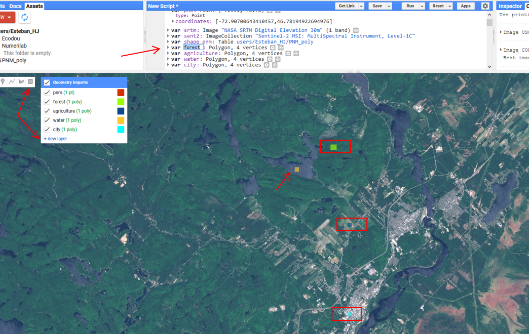
- The first manipulation is to build the training dataset. Use the geometry tool to create polygons. Be careful to use a small area to avoid script error when you run the code. Helped by the geometry tool, draw a polygon in a forested area and rename it “forest” in your script. Repeat this step for polygons in agricultural, water and urban landscapes. Rename those polygons respectively “agriculture”, “water” and “city”.
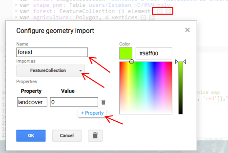
- Next, you need to add a label to each polygon in the same way you would create an attribute column in an attribute table of a shapefile. Those labels will be useful when you will merge all polygons together. To add a label, open polygons propriety –> select “FeatureCollection” –> Add property –> Name it “landcover” –> Give it a value of 0 (number zero) –> Ok. Do this step for the others polygons with values of 1-2 and 3 respectively. After this step, each polygon should be a FeatureCollection object.
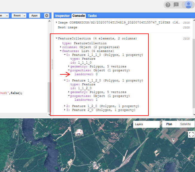
- Use the following code to merge polygons together and print it in the console.
// Merge polygons together
var classNames = forest.merge(agriculture).merge(water).merge(city);

print(classNames);
- Now you can use classNames layers to create the training data. This training data will associate different band values from an image to the polygon you drew. Here we use bands 2,3,4 and 8 (RGB and NIR bands that have a 10m resolution).
var bands = ['B2', 'B3', 'B4', 'B8']; // Define the bands to use for the classification

// Create the training dataset
var training = pnm_i.select(bands).sampleRegions({
  collection: classNames,
  properties: ['landcover'],
  scale: 30
});

print(training, 'training dataset');
- Now you can test the classification for the entire satellite image.
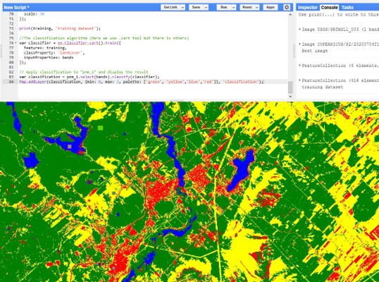
//The classification algorithm (Here we use .cart tool, but there are others)
var classifier = ee.Classifier.smileCart().train({
  features: training,
  classProperty: 'landcover',
  inputProperties: bands
});

// Apply classification to "pnm_i" and display the result
var classification = pnm_i.select(bands).classify(classifier);
Map.addLayer(classification, {min: 0, max: 3, palette: ['green', 'yellow','blue','red']}, 'classification');
- This first classification is not perfect. For example, one mistake from the classification is that there is too much agricultural landscape compared to reality. To make the classification more accurate, you could add NDVI data that you created earlier. To do so, you will need to use your created object “ndvi1” that contains ndvi index and satellite image bands.
// Add other bands
var bands2 = ['B2', 'B3', 'B4', 'B8', 'NDVI']; // pour définir les bandes a utiliser
// Create a new training dataset with the new bands of ndvi1 object
var training2 = ndvi1.select(bands2).sampleRegions({
collection: classNames,
properties: ['landcover'],
scale: 30
});
// Classification algorithm
var classifier2 = ee.Classifier.smileCart().train({
features: training2,
classProperty: 'landcover',
inputProperties: bands2
});
// Apply classification to ndvi1 object and display the result
var classification2 = ndvi1.select(bands2).classify(classifier2);
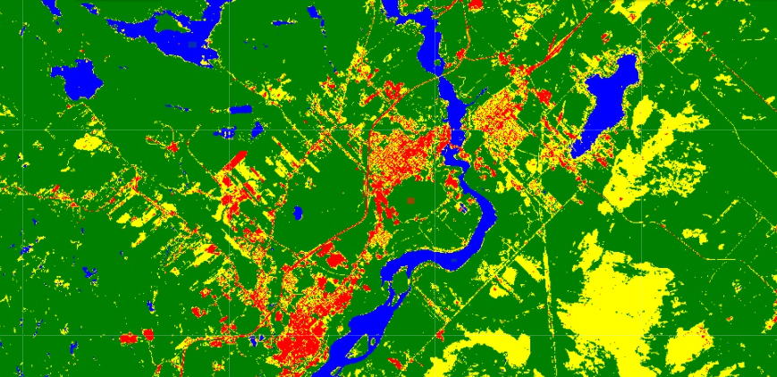
Map.addLayer(classification2, {min: 0, max: 3, palette: ['green', 'yellow','blue','red']}, 'classification +ndvi');
- The final image could look like that, but it is still not perfect.
Step 8: Export raster layer to Google Drive
It is possible to export the layer you created in GEE via Google Drive. From there, you can continue to modify those layers in a GIS software for example. In this step, you will export only a small region of the classification because the entire image would be too heavy to export.
- Start by adding a landmark that you will call “zone”.
- This code creates a buffer zone with a radius of 1500 meters around the landmark.
// Create an export zone with a buffer
var zone=zone.buffer(1500);
Map.addLayer(zone,rgb_colour,"Export zone");
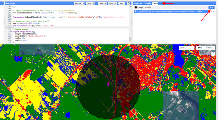
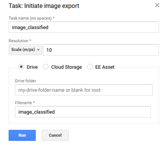
- You are now ready to export the classification layer for the buffer zone you defined previously in your Google Drive folder.
//Export raster
Export.image.toDrive({
  image: classification,
  description: 'image_classified',
  scale: 10,
  region: zone
});
- To finish exportation, click “run” in the task tab and adjust the export parameters as you desire. –> Run. In the following picture, everything is already fine so you can press “Run” right away without changing anything.
Step 9: Draw graph with GEE
GEE also allows you to create different type of charts to look at the distribution of the data. In this step, you will take the elevation layer that you will clip to La Mauricie National Park to create a chart about height distribution in this area.
- Create the elevation layer for the National Park area.
// Clip the elevation layer for the National Park
var elevation1= srtm.clip(shape_pnm);
print(elevation1,"Elevation 1");

// Check the result
Map.addLayer(elevation1, {min: 0, max: 400, palette: ['blue', 'yellow', 'red']},"Elevation colour pnm");
- Use the tool ui.Chart.image.histogram() to create a histogram that summarizes the distribution of heights in the National Park and print the result in the console. Other types of charts are available depending on the data you have and the type of graph you need.
// Draw a graph and print it in the console
var Chart1 = ui.Chart.image.histogram(
    elevation1,shape_pnm,30);
print(Chart1);
- It is also possible to add some visualization parameters to improve the look of the graph.
// Set some visualisation option to improve the look of the graph
var options = {
  title: "Height frequency distribution for La Mauricie National Park",
  fontSize: 15,
  hAxis: {title: "Elevation (m)"},
  vAxis: {title: 'Frequency'},
  series: {
    0: {color: 'magenta'}
  }};

// Create the improved graph
var Chart2 = ui.Chart.image.histogram(
    elevation1,shape_pnm,30)
    .setSeriesNames(['Height'])
    .setOptions(options);
print(Chart2);
- Once the graph is done, you can click on it in the console and from there it is possible to export these data in different formats. (Ex. .CSV)
End of the workshop