Mixed models with R
Marc Pépino
December 2022
- Introduction
- Packages
- Simple linear regression
- Mixed-models: varying-intercepts
- Mixed-models: varying-slopes
- LMM: brook charr allometry
- GLMM: brook charr abondance
- NLME: walleye growth curve
- References
Introduction
Linear mixed models (LMM) are natural extension of the simple linear regression and are now among the most standard and powerful techniques use to model ecological data. We first show this extension using simulations as I’m convinced that we well understand a model if we are able to simulate it. Simulations are also a precious help for teaching statistics. Using simulations, we wish to understand the output of mixed models that gives more information than the simple p-values, especially the variance structure of the data. We finally show how to apply mixed models to three cases studies, exploring linear mixed models and their extensions to generalized linear mixed models (GLMM) and non linear mixed models (NLME). At each step (i.e., data download, model fitting, model validation), we will use graphics to visualize what we have in hand. Without graphics, we walk blind and risk straying far from what we think we are modeling. We will explore LMM and their extensions using Pinheiro and Bates (2000) as the main reference book. Other complementary books include, but not limited to, Faraway (2006), Gelman and Hill (2006) for a soft transition to Bayesian modelling, and the Zuur et al. (2009) for practical applications of mixed models to ecological data and, probably, the most popular book consulted by students. An introduction to mixed models could also be found in articles like Wagner et al. (2006), Bolker (2009) or Harrison et al. (2018).
Packages
Wee need the following packages for this workshop. I’m usually as minimalist as possible and upload only the packages we really need. Be particularly careful to the order you upload the packages since some functions could be masked from package to package.
#Packages ####
library(ggplot2) #For graphic visualization
library(readxl) #For downloading Excel data
library(lme4) #For mixed models (most popular)
library(glmmTMB) #For speed up mixed models
library(nlme) #For mixed models (my favorite)
Simple linear regression
The simple linear regression is the starting point to understand mixed models. The regression line is defined by two parameters: the intercept (i.e., the y-value when x is equal to zero) and the slope (i.e., the increase of y when x increases from one unit). To simulate a simple linear regression, we also need to add residuals to y-values. This last step is the most important because it comes from the main assumption: residuals are independent and normally distributed with mean zero and variance ($\sigma^2$) to be estimated from the data. The equation of the simple linear regression could be written as follow:
\[y_i = \beta_0 + \beta_1 x_i + \epsilon_i, \epsilon_i \sim N(0,\sigma^2)\]Where $y_i$ and $x_i$ are variables, $\beta_0$ and $\beta_1$ are the parameters (i.e., the intercept and slope, respectively), and $\epsilon_i$ are the residuals.The index $i$ refers to observations.
We first define the parameters of the equation, then the predictor (i.e., x-values) and finally the response variable (i.e., y-values), adding the residuals with an additional parameter: the standard deviation (i.e., $\sigma$). In experimental studies, we can choose to have x-values coming from the uniform distribution. In observational studies, however, x-values generally come from the normal distribution. In this example, we will choose to have x-values coming from the normal distribution. Note that we also need to define how many observations we have in hand (i.e., the sample size: n).
Simulation
Note that in this simulation, we say that $y$ comes from the normal distribution with mean given by the linear equation,$\beta_0 + \beta_1 x$, and standard deviation coming from the residuals, which is equivalent to first add the linear equation and then the residuals.
# Define the parameters of the equation
b0 = 5 # Intercept
b1 = 3 # Slope
sigma = 30 #standard deviation of the residuals

# Define the data
n = 50 #Sample size
x = rnorm(n,mean=125,sd=10)
y = rnorm(n,mean=b0+b1*x,sd=sigma)
dat = data.frame(x,y)
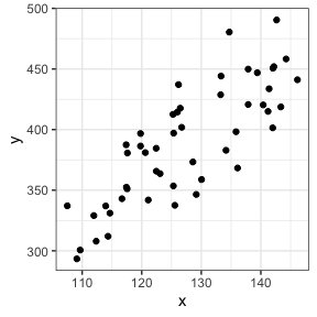
Graphic
Let’s take a look at our data
# Visualization
ggplot(data=dat,aes(x=x,y=y))+
  geom_point()+
  theme_bw()
Analyses
The code for model fitting is generally quite easy and the shortest part of the exercise.
mod = lm(y~x,data=dat)
Results
The summary function is usually used to explore the output of the model.
summary(mod)
Call:
lm(formula = y ~ x, data = dat)

Residuals:
   Min     1Q Median     3Q    Max
-51.45 -23.78  -3.68  19.78  65.68

Coefficients:
            Estimate Std. Error t value Pr(>|t|)
(Intercept) -68.6240    47.3891  -1.448    0.154
x             3.5884     0.3705   9.685 7.15e-13 ***
---
Signif. codes:  0 '***' 0.001 '**' 0.01 '*' 0.05 '.' 0.1 ' ' 1

Residual standard error: 28.3 on 48 degrees of freedom
Multiple R-squared:  0.6615,	Adjusted R-squared:  0.6544
F-statistic:  93.8 on 1 and 48 DF,  p-value: 7.147e-13
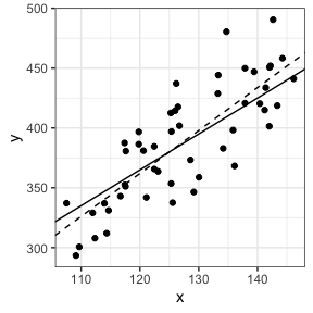
In this example, we see the intercept, the slope (x), but also the estimated standard deviation of the residuals (Residual standard error) and how the variance is explained by the predictor (Multiple R-squared, i.e., the coefficient of determination, $R^2$). We can see that the parameter values are closed of what we have simulated but not exactly the same, especially for the intercept. This is what we expect since we add residuals to y-values. Increasing residuals (i.e., increasing sigma in simulating data) leads to lower fit.
Let’s take a look at our data, adding simulated (solid) and estimated (broken) lines.
# Visualization
ggplot(data=dat,aes(x=x,y=y))+
  geom_abline(intercept=b0,slope=b1)+
  geom_abline(intercept=coef(mod)[1],slope=coef(mod)[2],lty=2)+
  geom_point()+
  theme_bw()
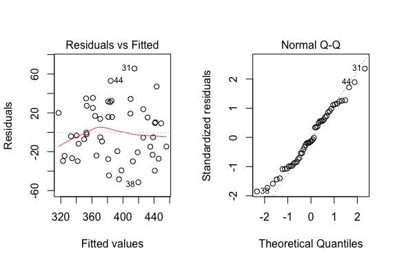
Assumptions
The first plot is to verify the independence of the data and the homogeneity of the residuals. The second plot is to verify the normality of the residuals.
# Model checking
par(mfrow=c(1,2))
plot(mod,which=c(1,2))
Mixed-models: varying-intercepts
The simplest LMM is the varying-intercept model. Because of the presence of grouped data, the main assumption of the independence of the data is violated. Then, LMM comes from a natural extension of the linear regression, assuming than the intercept could vary among groups. This variation is assumed to come from a normal distribution, with mean zero and variance (i.e., $\sigma_{\beta0}^2$) to be estimated from the data. In this way, we obtain a global relationship at the population level (i.e., fixed effects) and deviation at the group level (i.e. random effects).
The equation of LMM with varying-intercept could be written in two steps:
\[y_{ij} = \beta_{0j} + \beta_1 x_{ij} + \epsilon_{ij}, \epsilon_{ij} \sim N(0,\sigma^2)\] \[\beta_{0j} = \beta_0 + b_{0j}, b_{0j} \sim N(0,\sigma_{\beta0}^2)\]Where $y_{ij}$ and $x_{ij}$ are variables, $\beta_0$ and $\beta_1$ are the parameters (the intercept and slope, respectively) at the population level, $\beta_{0j}$ are the intercepts at the group level, $b_{0j}$ are the group level residuals of the intercept, and $\epsilon_{ij}$ are the level-one residuals.The index $j$ refers to group level. The index $i$ refers to observations.
Simulation
To simulate LMM, we need an additional parameter, the standard deviation of the intercept at the group level (i.e., $\sigma_{\beta0}$). Since we need to simulate the data at each group level,we will define the x-values for each group and then loop the simulation for all groups.
# Define the parameters of the equation
b1 = 3 #slope
b0 = 5 #intercept
sigma = 10 #sd for residuals
sigmab0 = 20 #sd for intercepts
b0j = rnorm(n=1000,mean=0,sd=sigmab0)

# Define the data
ng = 10 #number of group
nj = sample(20:40,ng,replace=TRUE) #sample size in each group
xmean = runif(ng,-25,25) #x mean in each group
xsd = runif(ng,5,10) #x sd in each group

# Loop for all groups
dat = data.frame()
for(j in 1:ng){
  x = rnorm(nj[j],mean=xmean[j],sd=xsd[j])
  y = rnorm(nj[j],mean=b0+b0j[j]+b1*x,sd=sigma)
  g = rep(j,nj[j])
  dat = rbind(dat,data.frame(x,y,g))
}

dat$g = as.factor(dat$g)
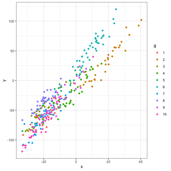
Graphic
Let’s take a look at our data
#Visualization
ggplot(data=dat,aes(x=x,y=y,col=g))+
  geom_point()+
  theme_bw()
Analyses
Traditionally we could analyse this type of data using ANCOVA, using the grouping factor as an additional predictor. However, a more powerful technique is to use LMM with varying-intercept. Using the nlme package, the random argument specifies the intercept (i.e., 1) and the grouping factor (i.e., g in this example) as follow:
#Analyses: ANCOVA
mod = lm(y~x+g,data=dat)
summary(mod)
Call:
lm(formula = y ~ x + g, data = dat)

Residuals:
     Min       1Q   Median       3Q      Max
-23.7049  -6.1446   0.3523   6.7870  26.3402

Coefficients:
             Estimate Std. Error t value Pr(>|t|)
(Intercept)  -4.58808    2.32945  -1.970 0.049769 *
x             3.04646    0.07239  42.084  < 2e-16 ***
g2          -20.59491    3.71571  -5.543 6.35e-08 ***
g3           15.36780    2.61833   5.869 1.12e-08 ***
g4           -9.37524    2.80239  -3.345 0.000922 ***
g5           15.12837    2.84610   5.315 2.03e-07 ***
g6           29.96195    3.27074   9.161  < 2e-16 ***
g7            2.48753    2.54925   0.976 0.329926
g8           28.64816    2.59083  11.058  < 2e-16 ***
g9            2.40887    2.76159   0.872 0.383729
g10          -1.18766    2.62787  -0.452 0.651621
---
Signif. codes:  0 '***' 0.001 '**' 0.01 '*' 0.05 '.' 0.1 ' ' 1

Residual standard error: 9.788 on 312 degrees of freedom
Multiple R-squared:   0.96,	Adjusted R-squared:  0.9587
F-statistic: 749.1 on 10 and 312 DF,  p-value: < 2.2e-16
#Analyses: Mixed models with nlme package
mod = lme(y~x,random=~1|g,data=dat)
summary(mod)
Linear mixed-effects model fit by REML
  Data: dat
       AIC      BIC    logLik
  2439.092 2454.178 -1215.546

Random effects:
 Formula: ~1 | g
        (Intercept) Residual
StdDev:    15.93838 9.787311

Fixed effects:  y ~ x
               Value Std.Error  DF  t-value p-value
(Intercept) 1.601332  5.110372 312  0.31335  0.7542
x           3.035387  0.071049 312 42.72226  0.0000
 Correlation:
  (Intr)
x 0.125

Standardized Within-Group Residuals:
        Min          Q1         Med          Q3         Max
-2.41041756 -0.62668163  0.03215744  0.70114206  2.67355343

Number of Observations: 323
Number of Groups: 10
The interpretation of the ANCOVA could be tedious, especially as the number of groups increases. The interpretation of the mixed model is more straightforward, at least for the fixed effects…
Results
We can easily retrieve the summary output using different functions and compare the results to simulated parameters. This exercise is particularly helpful to see how well the model fits to the data. This could be helpful, for example, to found the best sampling design before collecting ecological data (e.g., Pépino et al. 2016). Especially, the intervals functions gives the confidence intervals of parameter estimates (the default is 95%), which can be used to report the final result of the model.
fixef(mod) #The coefficient of the fixed effects (estimates)
(Intercept)           x
   1.601332    3.035387
ranef(mod) #b0j estimates
   (Intercept)
1    -6.274000
2   -26.251615
3     8.845424
4   -15.420527
5     8.704950
6    23.639338
7    -3.881986
8    22.007652
9    -3.825922
10   -7.543314
VarCorr(mod) #the variance covariance structure (sigmab0 and sigma estimates)
g = pdLogChol(1)
            Variance  StdDev
(Intercept) 254.03190 15.938378
Residual     95.79145  9.787311
intervals(mod) #95 confidence intervals of parameter estimates
Approximate 95% confidence intervals

 Fixed effects:
                lower     est.     upper
(Intercept) -8.453819 1.601332 11.656483
x            2.895591 3.035387  3.175184

 Random Effects:
  Level: g
                   lower     est.    upper
sd((Intercept)) 9.976875 15.93838 25.46207

 Within-group standard error:
    lower      est.     upper
 9.048780  9.787311 10.586118
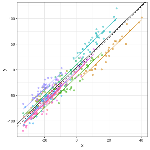
We can also add the fitted and residuals values to the original data frame using the fitted and residuals function, respectively. This is particularly helpful for checking model assumptions or illustrating model fitting. Here, black and color lines refer to regression lines at the population and group levels, respectively.
dat$fit = fitted(mod) #fitted values
dat$res = residuals(mod) #residuals values

# Visualization
ggplot(data=dat,aes(x=x,y=y,col=g))+
  geom_abline(intercept=b0,slope=b1)+
  geom_abline(intercept=fixef(mod)[1],slope=fixef(mod)[2],lty=2)+
  geom_point(alpha=0.5)+
  geom_line(aes(x=x,y=fit,col=g),linewidth=1)+
  #facet_wrap(~g)+ #Optional
  theme_bw()+
  theme(legend.position="none")
Assumptions
There are tow main assumptions.
Assumption 1: within-group errors
The within-group errors are independent and identically normally distributed, with mean zero and variance to be estimated, and they are independent of the random effects.
You can used default functions to verify this first assumption. Note that this assumption should be verify at the group level. You can also have an rough idea of the goodness-of-fit by plotting fitted versus observed values.
#Homogeneity of residuals
plot(mod)
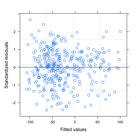
plot(mod,g~resid(.,type="p"),abline=0)
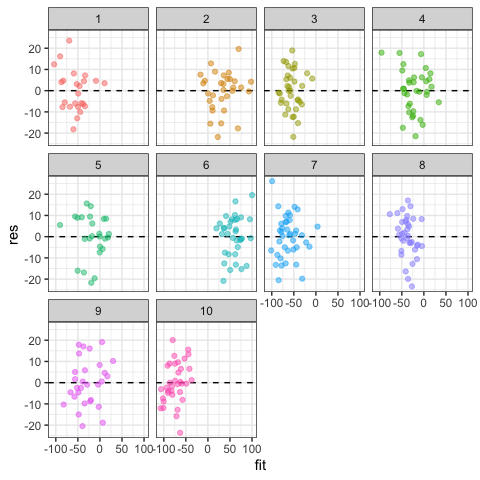
plot(mod,resid(.,type="p")~fitted(.)|g,abline=0,lty=2)
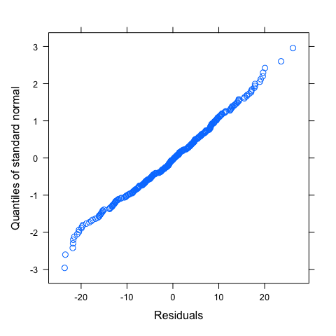
#Normality of residuals
qqnorm(mod,~resid(.))
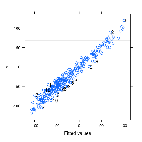
#Some idea of goodness-of-fit
plot(mod,y~fitted(.),id=0.05,adj=-0.3)
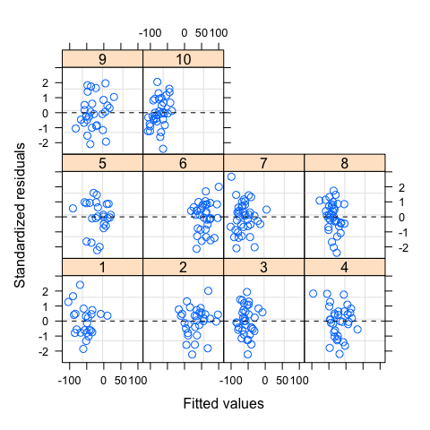
After adding residuals and fitted values to the data frame, you can also reproduce similar graphs using ggplot.
#Homogeneity of residuals
ggplot(data=dat,aes(x=fit,y=res,col=g))+
  geom_hline(yintercept=0,lty=2)+
  geom_point(alpha=0.5)+
  facet_wrap(~g)+
  theme_bw()+
  theme(legend.position="none")
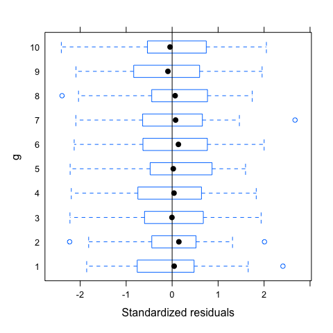
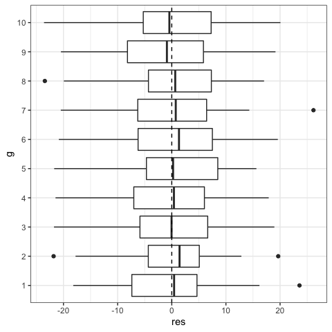
#Boxplot could also be used to see variation of residuals among groups
#You could also explore relationship between residuals and predictors
ggplot(data=dat,aes(x=g,y=res))+
  geom_boxplot()+
  geom_hline(yintercept=0,lty=2)+
  coord_flip()+
  theme_bw()
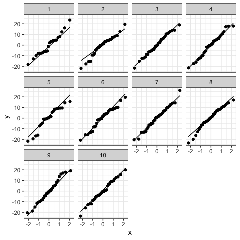
#Normality of residuals
ggplot(dat,aes(sample = res))+
  stat_qq()+
  stat_qq_line()+
  facet_wrap(~g)+#optional
  theme_bw()
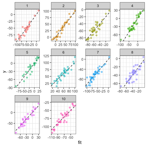
#Prediction: a rough idea of goodness-of-fit
ggplot(data=dat,aes(x=fit,y=y,col=g))+
  geom_abline(intercept=0,slope=1,lty=2)+
  geom_point(alpha=0.5)+
  facet_wrap(~g,scale="free")+
  theme_bw()+
  theme(legend.position="none")
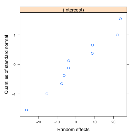
Assumption 2: random effects
The random effects are normally distributed, with mean zero and covariance matrix (not depending on the group) and are independent for different groups.
As before, you can use default functions or customize graphic output using ggplot. Note that with 10 groups, it is more difficult to evaluate carefully this second assumption.
#First option: default functions
#Normality of random effects
qqnorm(mod,~ranef(.))
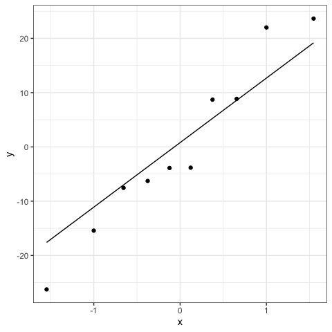
#Second option: ggplot
ran = ranef(mod)
ggplot(ran,aes(sample = ran[,1]))+
  stat_qq()+
  stat_qq_line()+
  theme_bw()
Violation of assumptions could include dependencies or heteroscedasticity among the within-group errors that can be modeled with correlation structure or the specification of the Variance-Covariance matrices for the random effects, respectively. Even if I encourage to adequately specify how to model the fixed and random effects, mixed models are generally robust to violations of these assumptions (Schielzeth et al. 2020).
Intraclass correlation
The intraclass correlation (ICC) is the proportion of the total variation that is among groups (Faraway 2006, Gelman and Hill 2007). The ICC could be calculated in varying-intercept models as follow:
\[\frac{\sigma_{\beta0}^2} {\sigma^2 + \sigma_{\beta0}^2}\]Where $\sigma^2 + \sigma_{\beta0}^2$ is the total variation and $\sigma_{\beta0}^2$, the variation among groups.
The ICC is thus the variation among groups divided by the total variation. The ICC ranges from 0 (all variation withing groups) to 1 (all variation among groups). You can read Reyjol et al. (2008) for an ecological application. Extension of ICC could also be found in animal behavior studies for the estimation of repeatability (e.g., Dingemanse and Dotcherman 2013, Allegue et al. 2017).
variation = as.numeric(VarCorr(mod)[,1])
ICC = variation[1]/sum(variation)
ICC
[1] 0.7261719
sigmab0^2/(sigmab0^2+sigma^2) #Predicted value of ICC based on simulated values
[1] 0.8
Mixed-models: varying-slopes
Now we can assume that not only the intercept could vary among groups, but also the slope. We could also assume that only the slope varies among groups and the intercept is fixed but, as many ecological data could vary both in intercept and slope, we will not explore this option here. This variation in slope is assumed to come from a normal distribution, with mean zero and variance ($\sigma_{\beta1}^2$) to be estimated from the data.
The equation of LMM with varying intercept and slope could be written as follow:
\[y_{ij} = \beta_{0j} + \beta_{1j} x_{ij} + \epsilon_{ij}, \epsilon_{ij} \sim N(0,\sigma^2)\] \[\beta_{0j} = \beta_0 + b_{0j}, b_{0j} \sim N(0,\sigma_{\beta0}^2)\] \[\beta_{1j} = \beta_1 + b_{1j}, b_{1j} \sim N(0,\sigma_{\beta1}^2)\]Where $y_{ij}$ and $x_{ij}$ are variables, $\beta_0$ and $\beta_1$ are the parameters (the intercept and slope, respectively) at the population level, $\beta_{0j}$ are the intercepts at the group level, $\beta_{1j}$ are the slopes at the group level, $b_{0j}$ are the group level residuals of the intercept, $b_{1j}$ are the group level residuals of the slope, and $\epsilon_{ij}$ are the level-one residuals.The index $j$ refers to group level. The index $i$ refers to observations. Important: random intercept and random slope are not assumed to be independent from each other, which is taking into account by their covariance matrix. For simplicity, we will assume that they are independent in the following simulations.
Simulations
The simulation look like the varying-intercept mixed model. The only difference is that we add an additional parameter, the standard deviation ($\sigma_{\beta1}$) to take into account that the slope could vary among groups.
dat = data.frame()

# Define the parameters of the equation
b1 = 3 #slope
b0 = 5 #intercept
sigma = 10 #sd for residuals
sigmab0 = 20 #sd for intercepts (try 20)
sigmab1 = 1 #sd for slopes (try 1 or 0.2 or 0)
b0j = rnorm(n=1000,mean=0,sd=sigmab0)
b1j = rnorm(n=1000,mean=0,sd=sigmab1)

# Define the data
ng = 10 #number of group
nj = sample(20:40,ng,replace=TRUE) #sample size in each group
xmean = runif(ng,-25,25) #x mean in each group
xsd = runif(ng,5,10) #x sd in each group try: (5,10) or (1) or 30

# Loop for all groups
dat = data.frame()
for(j in 1:ng){
  x = rnorm(nj[j],mean=xmean[j],sd=xsd[j])
  y = rnorm(nj[j],mean=b0+b0j[j]+(b1+b1j[j])*x,sd=sigma)
  g = rep(j,nj[j])
  dat = rbind(dat,data.frame(x,y,g))
}

dat$g = as.factor(dat$g)
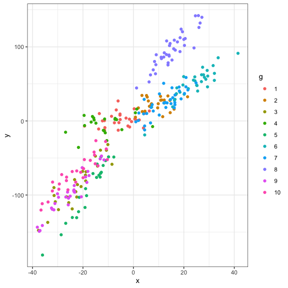
Graphic
Let’s take a look at our data
#Visualization
ggplot(data=dat,aes(x=x,y=y,col=g))+
  geom_point()+
  theme_bw()
Analyses
As for LMM with varying-intercept, we start with a model fitting using ANCOVA, but with an interaction term. The varying-slope model is specified by adding the predictor x in the random argument. Note that the ANCOVA output could be particularly difficult to interpret, especially as the number of groups increases. LMM output is more straightforward, with the same number of parameters whatever the number of groups.
# Analyses: ANCOVA
mod = lm(y~x*g,data=dat)
summary(mod)
Call:
lm(formula = y ~ x * g, data = dat)

Residuals:
    Min      1Q  Median      3Q     Max
-27.410  -6.494  -0.313   6.256  28.988

Coefficients:
            Estimate Std. Error t value Pr(>|t|)
(Intercept)   3.6850     2.4732   1.490  0.13742
x             0.4027     0.3120   1.291  0.19793
g2           14.7585     4.9330   2.992  0.00304 **
g3          -11.0255     6.7928  -1.623  0.10576
g4           -2.3594     4.5790  -0.515  0.60679
g5           -1.6848     6.5532  -0.257  0.79731
g6          -13.1434     6.5245  -2.014  0.04498 *
g7           -5.7461     4.4803  -1.283  0.20079
g8           39.8874     5.0984   7.824 1.25e-13 ***
g9          -11.9828     7.2724  -1.648  0.10061
g10         -10.5213     6.5113  -1.616  0.10732
x:g2          0.1196     0.5088   0.235  0.81440
x:g3          3.1410     0.4117   7.629 4.34e-13 ***
x:g4          0.1057     0.4168   0.253  0.80010
x:g5          4.9061     0.4472  10.971  < 2e-16 ***
x:g6          2.0745     0.3937   5.269 2.86e-07 ***
x:g7          1.7577     0.4126   4.260 2.85e-05 ***
x:g8          3.0249     0.4116   7.350 2.51e-12 ***
x:g9          3.1552     0.4059   7.773 1.73e-13 ***
x:g10         2.4086     0.4009   6.009 6.21e-09 ***
---
Signif. codes:  0 '***' 0.001 '**' 0.01 '*' 0.05 '.' 0.1 ' ' 1

Residual standard error: 10.17 on 263 degrees of freedom
Multiple R-squared:  0.9803,	Adjusted R-squared:  0.9789
F-statistic:   688 on 19 and 263 DF,  p-value: < 2.2e-16
# Analyses: Mixed models with nlme package - random intercept
mod0 = lme(y~x,random=~1|g,data=dat)
summary(mod0)
Linear mixed-effects model fit by REML
  Data: dat
       AIC      BIC    logLik
  2343.084 2357.637 -1167.542

Random effects:
 Formula: ~1 | g
        (Intercept) Residual
StdDev:    29.89671 13.88851

Fixed effects:  y ~ x
                Value Std.Error  DF   t-value p-value
(Intercept) -4.228197  9.504821 272 -0.444848  0.6568
x            2.619327  0.117580 272 22.276956  0.0000
 Correlation:
  (Intr)
x 0.053

Standardized Within-Group Residuals:
         Min           Q1          Med           Q3          Max
-3.791434759 -0.590994740 -0.006061655  0.640791495  2.420196655

Number of Observations: 283
Number of Groups: 10
# Analyses: Mixed models with nlme package - random intercept and slope
mod1 = lme(y~x,random=~x|g,data=dat)
summary(mod1)
Linear mixed-effects model fit by REML
  Data: dat
       AIC      BIC    logLik
  2197.994 2219.824 -1092.997

Random effects:
 Formula: ~x | g
 Structure: General positive-definite, Log-Cholesky parametrization
            StdDev    Corr
(Intercept) 15.847055 (Intr)
x            1.590983 -0.05
Residual    10.166360

Fixed effects:  y ~ x
               Value Std.Error  DF  t-value p-value
(Intercept) 3.512384  5.260836 272 0.667647  0.5049
x           2.513745  0.510795 272 4.921242  0.0000
 Correlation:
  (Intr)
x -0.036

Standardized Within-Group Residuals:
        Min          Q1         Med          Q3         Max
-2.76861646 -0.63737211 -0.02064573  0.62375233  2.86482177

Number of Observations: 283
Number of Groups: 10
Results
As for the varying-intercept mixed model, we can compare model estimates with simulated values using the same functions!
fixef(mod1) #The coefficient of the fixed effects (estimates)
(Intercept)           x
   3.512384    2.513745
ranef(mod1) #b0j estimates
   (Intercept)           x
1    0.5730601 -2.03206100
2   13.0055977 -1.80691304
3   -9.9867624  1.06178060
4   -1.3780864 -1.93847817
5   -3.1706913  2.69934276
6  -11.3913918 -0.09622784
7   -5.4006808 -0.36205703
8   37.5826831  1.04759948
9  -10.6252539  1.08523496
10  -9.2084743  0.34177928
VarCorr(mod1) #the variance covariance structure
g = pdLogChol(x)
            Variance   StdDev    Corr
(Intercept) 251.129159 15.847055 (Intr)
x             2.531227  1.590983 -0.05
Residual    103.354876 10.166360
intervals(mod1) #95 confidence intervals of parameter estimates
Approximate 95% confidence intervals

 Fixed effects:
                lower     est.    upper
(Intercept) -6.844750 3.512384 13.86952
x            1.508131 2.513745  3.51936

 Random Effects:
  Level: g
                        lower        est.      upper
sd((Intercept))     9.5512907 15.84705522 26.2926935
sd(x)               0.9850315  1.59098298  2.5696913
cor((Intercept),x) -0.6125874 -0.04963095  0.5467327

 Within-group standard error:
    lower      est.     upper
 9.334299 10.166360 11.072591
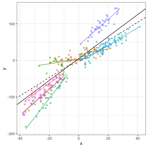
And the same code for plotting!
dat$fit = fitted(mod1) #fitted values
dat$res = residuals(mod1) #residuals values

# Visualization
ggplot(data=dat,aes(x=x,y=y,col=g))+
  geom_abline(intercept=b0,slope=b1)+
  geom_abline(intercept=fixef(mod1)[1],slope=fixef(mod1)[2],lty=2)+
  geom_point(alpha=0.5)+
  geom_line(aes(x=x,y=fit,col=g),linewidth=1)+
  #facet_wrap(~g)+ #Optional
  theme_bw()+
  theme(legend.position="none")
Testing random component
How to choose between random intercept or random slope models ? An easy way is to compare the two models using log-likelihood ratio test or comparing information criteria like Aikaike Information Criteria (AIC). Note that you have to use REML method to compare random effect and ML method to compare fixed effects (Zuur et al. 2009). You can also repeat the simulation using $\sigma_{\beta1} = 0.1$ and see if you obtain the same conclusion!
mod0 = lme(y~x,random=~1|g,data=dat,method="REML")
mod1 = lme(y~x,random=~x|g,data=dat,method="REML")
anova(mod0,mod1)
     Model df      AIC      BIC    logLik   Test  L.Ratio p-value
mod0     1  4 2343.084 2357.637 -1167.542
mod1     2  6 2197.994 2219.824 -1092.997 1 vs 2 149.0896  <.0001
A short note on grouped data. The groupedData function in the nlme package can be used to defined how your data are grouped and speed up model fitting and visualization. Grouped data are also useful to explore different structure of the variance-covariance matrix. In this simulation example, we did not assume any correlation between the slope and intercept of the random component, with can be specify using the pdDiag function. We repeat the preceding models, starting with the random intercept model and then updating this model using the update function. We then compare the models as before using the anova function.
#Grouped data and update function of the nlme package
datG = groupedData(y~x|g,data=dat)
mod0 = lme(y~x,random=~1|g,data=datG,method="REML")
mod1 = update(mod0,random=~x)
mod1diag = update(mod0,random=pdDiag(~x))
anova(mod0,mod1diag,mod1)
         Model df      AIC      BIC    logLik   Test   L.Ratio p-value
mod0         1  4 2343.084 2357.637 -1167.542
mod1diag     2  5 2196.014 2214.206 -1093.007 1 vs 2 149.06951  <.0001
mod1         3  6 2197.994 2219.824 -1092.997 2 vs 3   0.02011  0.8872
To be consistent with the simulation, you should select the model with the random slope and a diagonal variance-covariance matrix (i.e., mod1diag), but conclusions could differ depending of your simulated data…
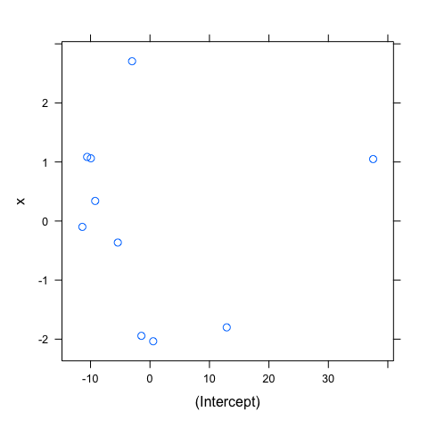
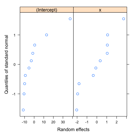
Assumptions
As for the varying-intercept model, the same assumptions applied and could be verify in the same way. You could thus verify these assumptions using the same code. I just show here the scatter plot of the estimated random effects. This plot is particularly useful to visualize the correlation between the intercept and slope of the random component, suggesting which variance-covariance matrix should be used. I also reproduce the normal Q-Q plots of the random effects to emphasize that the normality should be checked for both intercept and slope, but again, with only 10 groups, this assumption is difficult to verify.
#Correlation between random effects
pairs(mod1diag,~ranef(.))
#Normality of random effects
qqnorm(mod1diag,~ranef(.))
Further readings
How total variation in LMM is explained is less straightforward than in linear regressions. For an overview of the indices and available tools, you can consult Nakagawa and Schielzeth (2013), Johnson (2014),or Nakagawa et al. (2017).
How to well include the hierarchical structure of your data (e.g. nested or crossed design), you can consult Schielzeth and Nakagawa (2013) or Harrison et al. (2018).
Finally, before to explore how to fit mixed models to case studies, it is important to read Zuur et al. (2016), a practical guide for conducting and presenting results of regression-types analyses (e.g., see Fig. 1 in the original article). We outline here that model fitting arrives only at the step 6 (among the 10 steps recommended). Thinking (and stating) a relevant ecological question (step 1) and ensuring we have the right data in hand to answer it (step 2) are the primary initial steps that any statistical models can compensate…
LMM: brook charr allometry
The database could be found here: https://datadryad.org/stash/dataset/doi:10.5061/dryad.p2k02
In this example, we will explore the relationship between total length and mass in brook charr. Details of the sampling design could be found in the original article (Pépino et al. 2018). In brief, height families were raised in laboratory and were placed in lake enclosures for growth in summer in two distinct habitats (i.e., littoral or pelagic habitats).
Download and explore data
dat = read_excel("Data/Pepino_et_al_Original_Data.xlsx")

#Transform the total length and mass variables
dat$log10TL = log10(dat$Length_Final)
dat$log10M = log10(dat$Mass_Final)

datG = groupedData(log10M~log10TL|Family,data=dat)

#Visualization
ggplot(data=datG,aes(x=log10TL,y=log10M,col=Family))+
  geom_point()+
  facet_wrap(~Family)+
  theme_bw()

Blind linear mixed model
Many students try the simplest linear mixed model, taking into account the non-independence of the data. We will see how to go further in modelling the variability of ecological data.
#Analyses
mod0 = lme(log10M~log10TL,random=~1|Family,data=datG)

#Results
summary(mod0)
Linear mixed-effects model fit by REML
  Data: datG
       AIC       BIC  logLik
  -1778.77 -1762.487 893.385

Random effects:
 Formula: ~1 | Family
        (Intercept)  Residual
StdDev:  0.01990289 0.0297343

Fixed effects:  log10M ~ log10TL
                Value  Std.Error  DF   t-value p-value
(Intercept) -4.862396 0.05393961 426 -90.14519       0
log10TL      2.881259 0.02784003 426 103.49337       0
 Correlation:
        (Intr)
log10TL -0.991

Standardized Within-Group Residuals:
        Min          Q1         Med          Q3         Max
-5.66116458 -0.54323068 -0.03043674  0.53004392  5.58488220

Number of Observations: 435
Number of Groups: 8
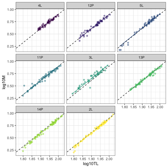
Let’s take a look at our data, adding the population (broken) and family-specific (solid) regression lines.
#Visualization
datG$fit = fitted(mod0)
datG$res = residuals(mod0)
ggplot(data=datG,aes(x=log10TL,y=log10M,col=Family))+
  geom_abline(intercept=fixef(mod0)[1],slope=fixef(mod0)[2],lty=2)+
  geom_point(alpha=0.5)+
  geom_line(aes(y=fit),linewidth=1)+
  facet_wrap(~Family)+ #Optional
  theme_bw()+
  theme(legend.position="none")
Do we stop the modelling here ?
Assumptions
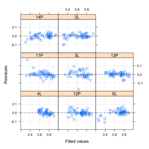
We can’t stop without checking at the assumptions of the model. We first check for the homogeneity of residuals.
#Homogeneity of residuals
plot(mod0,resid(.)~fitted(.)|Family,abline=0,lty=2)
Do we stop the modelling here ?
Random effects
The last plots show patterns in residuals. For example, residuals seem to increase with fitted values for families 14P and 5L, and decrease for family 4L, suggesting that including random slope in model could be useful to improve model fit. This graphical approach could be confirmed by testing the random component according to the approach suggested by Zuur et al. (2009). Following the Zuur’s approach, we start with the full model (i.e., including all variables with their interaction) and test to the random component (i.e., intercept and slope) with the REML method. Technically, model comparison or graphical inspection of the residuals should converge to the same specification of the final model.
modfullI = lme(log10M~log10TL*Zone,random=~1|Family,data=datG)
modfullS = lme(log10M~log10TL*Zone,random=~log10TL|Family,data=datG)
anova(modfullI,modfullS)
         Model df       AIC       BIC   logLik   Test  L.Ratio p-value
modfullI     1  6 -1842.539 -1818.142 927.2695
modfullS     2  8 -1869.018 -1836.490 942.5092 1 vs 2 30.47943  <.0001
Both AIC and log-likelihood ratio test show that we should include random slope.
Do we stop the modelling here ?
Fixed effects
Following the Zuur’s approach, we continue with comparing competing models differing in their fixed component using the ML method.
mod0 = lme(log10M~log10TL,random=~log10TL|Family,data=datG,method="ML")
mod1 = lme(log10M~log10TL+Zone,random=~log10TL|Family,data=datG,method="ML")
mod2 = lme(log10M~log10TL*Zone,random=~log10TL|Family,data=datG,method="ML")
anova(mod0,mod1,mod2)
     Model df       AIC       BIC   logLik   Test  L.Ratio p-value
mod0     1  6 -1825.685 -1801.233 918.8425
mod1     2  7 -1887.127 -1858.600 950.5635 1 vs 2 63.44192  <.0001
mod2     3  8 -1893.485 -1860.883 954.7427 2 vs 3  8.35833  0.0038
Both AIC and log-likelihood ratio test show that Model 2, including the two variables and their interaction, is the best model.
Do we stop the modelling here ?
Modelling heteroscedasticity
Let’s take a look at the homogeneity of the residuals.
mod2 = lme(log10M~log10TL*Zone,random=~log10TL|Family,data=datG,method="REML")
plot(mod2,resid(.,type="p")~fitted(.),abline=0,lty=2)
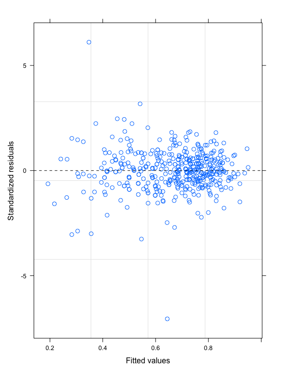
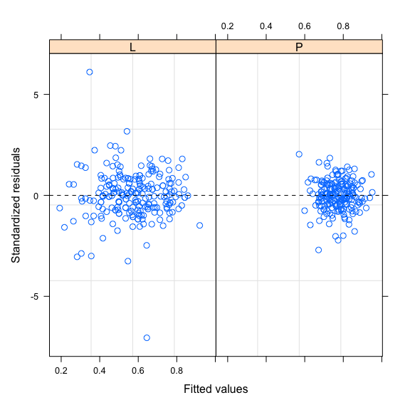
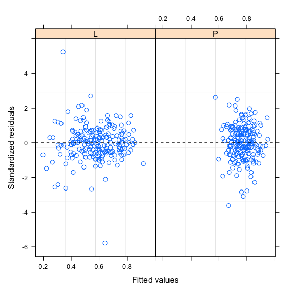
This plot shows that the variability of the residuals is higher for low fitted values, meaning heteroscedasticity of the residuals. This heteroscedasticity seems to come from different variation of the residuals according to the Zone variable, as shown in the plot below:
plot(mod2,resid(.,type="p")~fitted(.)|Zone,abline=0,lty=2)
We can model this heteroscedasticity using the weights argument and the varIdent function as follow:
mod2H = lme(log10M~log10TL*Zone,random=~log10TL|Family,data=datG,method="REML",
            weights = varIdent(form = ~ 1|Zone))

anova(mod2,mod2H)
      Model df       AIC       BIC   logLik   Test L.Ratio p-value
mod2      1  8 -1869.018 -1836.490 942.5092
mod2H     2  9 -1915.376 -1878.781 966.6881 1 vs 2 48.3578  <.0001
plot(mod2H,resid(.,type="p")~fitted(.)|Zone,abline=0,lty=2)
Model comparison based on AIC and log-likelihood ratio test show that modelling heteroscedasticity improves model fit. Residual variability is also more homogeneous in the two habitats. After choosing the better random and fixed components and including the Zone variable to model heteroscedasticity, we now have a model that better captures the data variability. We can stop the modelling here.
Results
We can then report the results of the best model, first by reporting the parameter estimates and their confidence intervals and then illustrating this result on a plot.
intervals(mod2H)
Approximate 95% confidence intervals

 Fixed effects:
                   lower       est.      upper
(Intercept)   -5.6004388 -5.3142985 -5.0281581
log10TL        2.9775185  3.1252230  3.2729275
ZoneP          0.1992625  0.4801723  0.7610822
log10TL:ZoneP -0.4086951 -0.2628585 -0.1170220

 Random Effects:
  Level: Family
                               lower       est.      upper
sd((Intercept))           0.16999148  0.3152096  0.5844827
sd(log10TL)               0.08573837  0.1596196  0.2971647
cor((Intercept),log10TL) -0.99974099 -0.9986156 -0.9926182

 Variance function:
      lower     est.     upper
P 0.5294444 0.607688 0.6974946

 Within-group standard error:
     lower       est.      upper
0.02826388 0.03110539 0.03423257
This case study shows us how to model and interpret more than the fixed effects, especially how the variation could be explained. For example, the variance function tells us that the variation in the pelagic habitat is 0.6 times the variation in the littoral habitat. Modeling the variation of ecological data gives us a more complete understanding of the ecological processes at work.
# Visualization
datG$fit = predict(mod2H)
datG$res = residuals(mod2H)
ggplot(data=datG,aes(x=log10TL,y=log10M,col=Zone))+
  geom_point(alpha=0.5)+
  geom_line(aes(y=fit),linewidth=1)+
  facet_wrap(~Family)+ #Optional
  theme_bw()
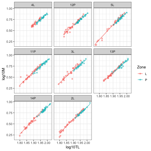
This best model shows that we have a random variation of the length-mass relationship according to the family and that this relationship is different in the two types of habitat, the slope being slower in the pelagic habitat. We finish, however, with a general though: is the length-mass relationship is really different according to the habitat type or, alternatively, the relationship shift according to the size (total length) of the individual? Since the overlap of total length according to the habitat is low, we can completely distinguish these two possible explanations. This outlines the importance to have the right data in hand to answer ecological question.
GLMM: brook charr abondance
The database could be found here: https://datadryad.org/stash/landing/show?id=doi%3A10.5061%2Fdryad.34tmpg4p8
In this case study, we will explore the relative abundance of brook charr in littoral habitat of Canadian Shield lakes. Details of the sampling design could be found in the original article (Rainville et al. 2022). In brief, brook charr were captured in 24 lakes and three consecutive years. This sampling design is thus typical of crossed design, year and lake including as random effects. We will focus here on the distribution of the response variable, extending LMM to GLMM.
Download and explore data
dat = read_excel("Data/Data_Rainville_et_al_2022_Evolutionary_Ecology.xlsx",
sheet = "BDlittoral")
dat$Temp = dat$T #Temperature variable
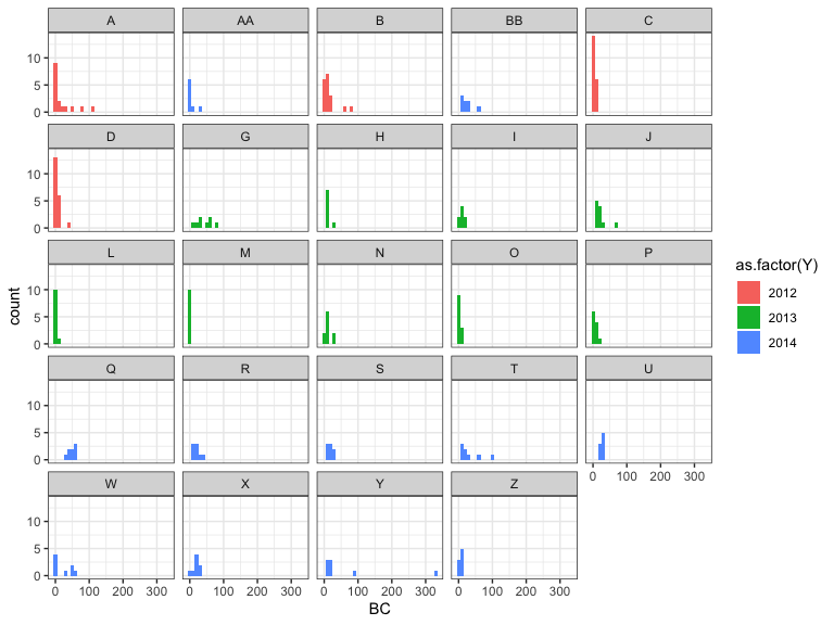
#Visualization: distribution of captures
ggplot(data=dat,aes(x=BC,fill=as.factor(Y)))+
geom_histogram(binwidth=10)+
facet_wrap(~LC)+
theme_bw()
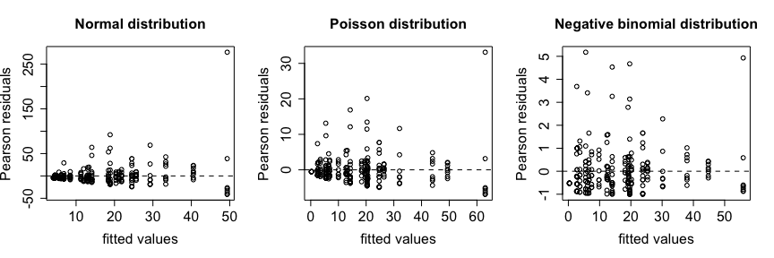
Negative binomial distribution
We will use the lme4 package. We don’t explore the influence of predictors in this example, but we will show how to deal with crossed design that is quite straightforward using lme4 package. Extending LMM to GLMM is also straightforward using the family argument to specify the distribution of the response variable. Since the response variable are the number of captures, appropriate distributions could be the Poisson or the negative binomial distributions. The negative binomial distribution can generally handle the overdispersion of ecological data and is often more appropriate than the Poisson distribution. As before, the two models can be compare using the anova function. For simplicity, we will not explore the potential relationship with the predictors (e.g., the temperature). Note that simulated values from LMM (i.e., normal distribution) are obtained with the simulate function and could be negative, which is not possible (number of captures cannot be negative). The negative distribution simulates more high abundances than the Poisson distribution.
#Normal distribution
mod.N = lmer(BC~1+(1|LC)+(1|Y),data=dat)
simulate(mod.N,nsim=5)[1:10,1:5]
       sim_1       sim_2      sim_3      sim_4     sim_5
1  22.177275 -49.4177181  56.271410  34.687981 72.073170
2  17.024076  -0.1053373   5.234417  31.821681 33.430622
3  51.075015 -24.4760264  -5.222976 -10.643936 29.809958
4  -1.090146  15.3458591  16.145508 -10.633513 39.518018
5  38.434107  35.7595436  32.733063   8.619748 26.227723
6  -2.585815 -42.0272885  32.300223 -31.156558 43.610788
7  53.544889  11.1338845  13.311571  -4.676094  2.509264
8  29.041403  -5.6599222 -10.201517  -2.191722 78.587746
9   8.483316  -2.4866802  48.440083  50.946557 46.433534
10 -7.191438  25.7922704   3.240183 -13.671578 38.992284
#Poisson distribution
mod.P = glmer(BC~1+(1|LC)+(1|Y),data=dat,family="poisson")
simulate(mod.P,nsim=5)[1:10,1:5]
   sim_1 sim_2 sim_3 sim_4 sim_5
1     18   112     4    14    10
2     18    97     3    15     8
3     14    90     3    18     6
4     22    93     2    16    12
5     16    82     2    15     8
6     24    80     2    20     6
7     21   105     5    12    10
8     29    87     2    17     4
9     13    88     5    14     8
10    14    82     1    18     5
#Negative binomial distribution
mod.NB = glmer.nb(BC~1+(1|LC)+(1|Y),data=dat)
simulate(mod.NB,nsim=5)[1:10,1:5]
   sim_1 sim_2 sim_3 sim_4 sim_5
1      3     3     2    12   113
2      3    38    40     8   577
3      1     6     5     1   166
4      1     3     1     2   202
5      4     7     3    16    43
6      0     8     3     0   228
7      2    19    34    10   125
8      0     3    17     5   124
9      0     2    41     4    83
10     4     8    49    15   117
anova(mod.P,mod.NB)
Data: dat
Models:
mod.P: BC ~ 1 + (1 | LC) + (1 | Y)
mod.NB: BC ~ 1 + (1 | LC) + (1 | Y)
       npar    AIC    BIC   logLik deviance  Chisq Df Pr(>Chisq)
mod.P     3 4335.2 4345.8 -2164.62   4329.2
mod.NB    4 1789.7 1803.8  -890.86   1781.7 2547.5  1  < 2.2e-16 ***
---
Signif. codes:  0 '***' 0.001 '**' 0.01 '*' 0.05 '.' 0.1 ' ' 1
The negative binomial model outperforms the Poisson model. Plots of fitted values versus Pearson residuals show how residuals are reduced and better distributed for the negative binomial distribution.
You can use the summary function to look at the results of the model.
summary(mod.NB)
Generalized linear mixed model fit by maximum likelihood (Laplace
  Approximation) [glmerMod]
 Family: Negative Binomial(1.0623)  ( log )
Formula: BC ~ 1 + (1 | LC) + (1 | Y)
   Data: dat

     AIC      BIC   logLik deviance df.resid
  1789.7   1803.8   -890.9   1781.7      247

Scaled residuals:
    Min      1Q  Median      3Q     Max
-1.0084 -0.6210 -0.2681  0.3030  5.1776

Random effects:
 Groups Name        Variance Std.Dev.
 LC     (Intercept) 1.1406   1.0680
 Y      (Intercept) 0.1758   0.4193
Number of obs: 251, groups:  LC, 24; Y, 3

Fixed effects:
            Estimate Std. Error z value Pr(>|z|)
(Intercept)   2.3887     0.3419   6.987 2.82e-12 ***
---
Signif. codes:  0 '***' 0.001 '**' 0.01 '*' 0.05 '.' 0.1 ' ' 1
Looking at p-vales of the fixed effect is not very meaningful (i.e., abundances is different from 0), however random effect show that variability is higher among lakes than among years.
The predict function is useful to obtain predicted values from the fitting model. The type argument is used to specify that we want predicted values on the original scale (i.e., the number of capture) whereas the re.form argument specifies how to deal with the random component: NA if we want to omit random effect and predict on fixed effects only, NULL if we want to predict considering all random effects, or a specific formula to indicate which random effect to consider in prediction. Note how the expand.grid function can be used to create a new data frame by considering the combination of variables included in the model.
newDat <- with(dat, expand.grid(LC=unique(LC), Y=unique(Y)))
newDat$predFix = predict(mod.NB,type="response",newdata=newDat,re.form=NA) #No random component
newDat$predRan = predict(mod.NB,type="response",newdata=newDat,re.form=NULL) #Full random components
newDat$predLC = predict(mod.NB,type="response",newdata=newDat,re.form=~(1|LC)) #Random component: lakes
newDat$predY = predict(mod.NB,type="response",newdata=newDat,re.form=~(1|Y)) #Random component: years
newDat[1:48,]
   LC    Y  predFix    predRan     predLC     predY
1   A 2012 10.89913 19.6258884 21.9914088  9.726754
2  AA 2012 10.89913  3.6094518  4.0445013  9.726754
3   B 2012 10.89913 14.0246398 15.7150383  9.726754
4  BB 2012 10.89913 14.0658020 15.7611617  9.726754
5   C 2012 10.89913  2.7984814  3.1357841  9.726754
6   D 2012 10.89913  5.5530209  6.2223299  9.726754
7   G 2012 10.89913 45.0371770 50.4655356  9.726754
8   H 2012 10.89913 14.9966975 16.8042587  9.726754
9   I 2012 10.89913 11.6287999 13.0304263  9.726754
10  J 2012 10.89913 22.6479304 25.3776994  9.726754
11  L 2012 10.89913  3.1772991  3.5602609  9.726754
12  M 2012 10.89913  0.4347612  0.4871632  9.726754
13  N 2012 10.89913 14.6509346 16.4168208  9.726754
14  O 2012 10.89913  4.3643540  4.8903923  9.726754
15  P 2012 10.89913  7.8086182  8.7497958  9.726754
16  Q 2012 10.89913 26.4542222 29.6427659  9.726754
17  R 2012 10.89913 11.9237583 13.3609362  9.726754
18  S 2012 10.89913 11.3996388 12.7736442  9.726754
19  T 2012 10.89913 17.8290762 19.9780257  9.726754
20  U 2012 10.89913 14.9658550 16.7696988  9.726754
21  W 2012 10.89913 14.0658020 15.7611617  9.726754
22  X 2012 10.89913 10.7415264 12.0362091  9.726754
23  Y 2012 10.89913 33.0505303 37.0341310  9.726754
24  Z 2012 10.89913  4.4000789  4.9304231  9.726754
25  A 2014 10.89913 33.2131390 21.9914088 16.460708
26 AA 2014 10.89913  6.1083209  4.0445013 16.460708
27  B 2014 10.89913 23.7340752 15.7150383 16.460708
28 BB 2014 10.89913 23.8037344 15.7611617 16.460708
29  C 2014 10.89913  4.7359054  3.1357841 16.460708
30  D 2014 10.89913  9.3974474  6.2223299 16.460708
31  G 2014 10.89913 76.2169837 50.4655356 16.460708
32  H 2014 10.89913 25.3791007 16.8042587 16.460708
33  I 2014 10.89913 19.6795650 13.0304263 16.460708
34  J 2014 10.89913 38.3273788 25.3776994 16.460708
35  L 2014 10.89913  5.3769835  3.5602609 16.460708
36  M 2014 10.89913  0.7357518  0.4871632 16.460708
37  N 2014 10.89913 24.7939618 16.4168208 16.460708
38  O 2014 10.89913  7.3858515  4.8903923 16.460708
39  P 2014 10.89913 13.2146233  8.7497958 16.460708
40  Q 2014 10.89913 44.7688146 29.6427659 16.460708
41  R 2014 10.89913 20.1787268 13.3609362 16.460708
42  S 2014 10.89913 19.2917527 12.7736442 16.460708
43  T 2014 10.89913 30.1723709 19.9780257 16.460708
44  U 2014 10.89913 25.3269056 16.7696988 16.460708
45  W 2014 10.89913 23.8037344 15.7611617 16.460708
46  X 2014 10.89913 18.1780208 12.0362091 16.460708
47  Y 2014 10.89913 55.9318301 37.0341310 16.460708
48  Z 2014 10.89913  7.4463091  4.9304231 16.460708
glmmTMB is another powerful package for GLMMs. The formula is quite similar to the lme4 package. You can consult the vignettes associated to this package for more details.
mod.P = glmmTMB(BC~1+(1|LC)+(1|Y),data=dat,family=poisson)
Binomial distribution
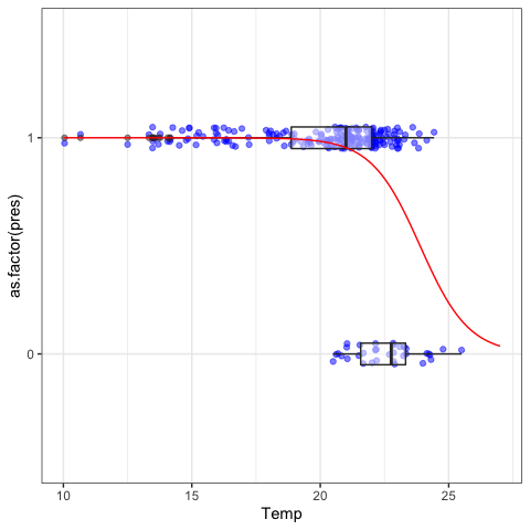
When the response variable is binary (e.g., presence/absence), the binomial distribution should be used. Here, we first transform the number of captures to a dummy variable (0 = no capture; 1: at least one capture). We then try to predict the probability to capture a brook charr in littoral habitat according to the temperature of the epilimnion (Temp variable).
dat$pres = ifelse(dat$BC==0,0,1)

#Analyses
mod.B = glmer(pres~Temp+(1|LC)+(1|Y),data=dat,family="binomial")

#Results
summary(mod.B)
Generalized linear mixed model fit by maximum likelihood (Laplace
  Approximation) [glmerMod]
 Family: binomial  ( logit )
Formula: pres ~ Temp + (1 | LC) + (1 | Y)
   Data: dat

     AIC      BIC   logLik deviance df.resid
   149.7    163.8    -70.9    141.7      247

Scaled residuals:
    Min      1Q  Median      3Q     Max
-4.3185  0.0232  0.1560  0.3582  1.2745

Random effects:
 Groups Name        Variance Std.Dev.
 LC     (Intercept) 1.5492   1.2447
 Y      (Intercept) 0.5855   0.7652
Number of obs: 251, groups:  LC, 24; Y, 3

Fixed effects:
            Estimate Std. Error z value Pr(>|z|)
(Intercept)  25.1542     6.2234   4.042  5.3e-05 ***
Temp         -1.0531     0.2784  -3.782 0.000155 ***
---
Signif. codes:  0 '***' 0.001 '**' 0.01 '*' 0.05 '.' 0.1 ' ' 1

Correlation of Fixed Effects:
     (Intr)
Temp -0.995
Temperature is highly significant, the coefficient being negative means that the probability of capturing a brook charr decreases as temperature increases. We can see this relationship on a plot.
#Visualization
newDat <- data.frame(Temp=seq(10,27,0.1))
newDat$predFix = predict(mod.B,type="response",newdata=newDat,re.form=NA)
newDat$x = 1 + newDat$predFix #just to add line on ggplot

ggplot(dat,aes(x=as.factor(pres),y=Temp))+
  geom_jitter(col="blue",position=position_jitter(0.05),alpha=0.5)+
  geom_boxplot(width=0.1,alpha=0.5)+
  geom_line(data=newDat,aes(x=x,y=Temp),col="red")+
  coord_flip()+
  theme_bw()
NLME: walleye growth curve
The database could be found here: https://datadryad.org/stash/dataset/doi:10.5061/dryad.vb957
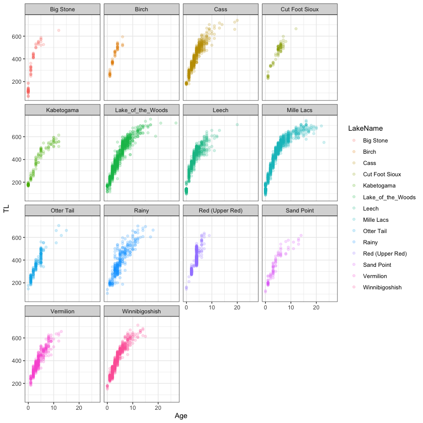
In this third case study, we will extend the conceptual framework of fixed and random effects in the context of non linear mixed models using the nlme package. This is particularly helpful to fit theoretical models to ecological data. We illustrate the use of NLME by fitting von Bertalanffy growth curve (VBGF) on walleye data. Extensive analyses of the walleye growth curve could be found in the original article (Honsey et al. 2017).
Download and explore data
dat = read_excel("Data/MN_Walleye_data_Honsey_et_al_Ecol_Apps.xlsx",sheet="Data")

dat$TL = dat$TotalLength

dat = dat[,-c(6,7)] #Remove Sex and Maturity that contain missing values

datG = groupedData(TL~Age|LakeName,data=dat)

#Visualization
ggplot(data=dat,aes(x=Age,y=TL,col=LakeName))+
  geom_point(alpha=0.2)+
  facet_wrap(~LakeName)+
  theme_bw()
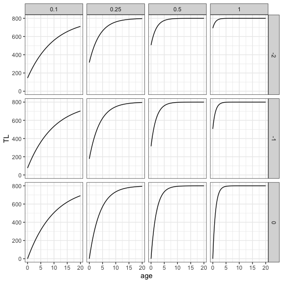
VBGF
The VBGF is defined by three parameters: Linf, the asymptotic length, k, the growth coefficient, and t0, the theoretical age when size (total length) equals zero. The best way to understand how these parameters influence the VBGF is to first define the VBGF function and then visualize the growth curve for different values of the parameters. On the plot below, Linf is fixed to 800, k, ranges from 0.1 to 1 and t0, from -2 to 0.
#Define the von Bertalanffy function

VBGF = function(x,Linf,k,t0) Linf*(1-exp(-k*(x-t0)))

#Visualization
age = seq(0,20,0.1)
k = c(0.1,0.25,0.5,1)
t0 = c(-2,-1,0)
newDat = expand.grid(age=age,k=k,t0=t0)
newDat$TL = VBGF(x=newDat$age,Linf=800,k=newDat$k,t0=newDat$t0)

ggplot(data=newDat,aes(x=age,y=TL))+
  geom_line(linewidth=1)+
  facet_grid(t0~k)+
  theme_bw()
## Warning: Ignoring unknown parameters: linewidth
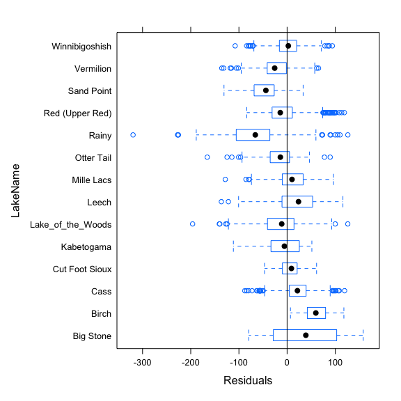
nls and nlsList
The nls function can fit non linear model. Plotting the residuals according to the grouping variable informs us how it is important to incorporate the random effects to the model. Here, we see that residuals are not centered to zero for many lakes, indicating biases in model fit. Random effects have to be included in the model to improve model fit.
#nls
mod.nls = nls(TL~VBGF(Age,Linf,k,t0),data=dat,
              start=c(Linf=800,k=.3,t0=-2))
summary(mod.nls)
Formula: TL ~ VBGF(Age, Linf, k, t0)

Parameters:
      Estimate Std. Error t value Pr(>|t|)
Linf 686.20487    3.84292  178.56   <2e-16 ***
k      0.18346    0.00264   69.50   <2e-16 ***
t0    -1.31013    0.02532  -51.75   <2e-16 ***
---
Signif. codes:  0 '***' 0.001 '**' 0.01 '*' 0.05 '.' 0.1 ' ' 1

Residual standard error: 42.74 on 6232 degrees of freedom

Number of iterations to convergence: 4
Achieved convergence tolerance: 8.025e-06
plot(mod.nls,LakeName~resid(.),abline=0)
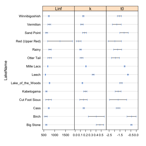
The nlsList function from the nlme package fits the non linear model by group and can be used to feed the NLME model. Plotting the estimates and confidence intervals of the parameters informs us which of the parameters should be incorporated to random effect into the model.
#nlsList
mod.lis = nlsList(TL~VBGF(Age,Linf,k,t0)|LakeName,data=dat,
                  start=c(Linf=800,k=.3,t0=-2))
mod.lis
Call:
  Model: TL ~ VBGF(Age, Linf, k, t0) | LakeName
   Data: dat

Coefficients:
                       Linf          k         t0
Big Stone          615.2847 0.47640877 -0.4496596
Birch              599.2751 0.40639674 -0.4326197
Cass               730.2746 0.16582262 -1.6728568
Cut Foot Sioux     721.9514 0.16013094 -1.6658202
Kabetogama         619.5719 0.19482829 -1.6663531
Lake_of_the_Woods  763.7969 0.13920308 -1.4058217
Leech              574.3497 0.34585097 -0.7668472
Mille Lacs         685.0770 0.20748989 -1.0721370
Otter Tail         768.9445 0.12378024 -1.9103712
Rainy              784.8787 0.10368433 -1.7118710
Red (Upper Red)   1246.5037 0.06944248 -1.9706741
Sand Point         628.2803 0.17967672 -1.1223282
Vermilion          752.8391 0.13023880 -1.7898292
Winnibigoshish     733.2848 0.15629007 -1.5480317

Degrees of freedom: 6235 total; 6193 residual
Residual standard error: 33.61449
plot(intervals(mod.lis),layout=c(3,1))
nlme
Since all the three parameters seem to vary by lake, we can fit the NLME with random effects for the three parameters. We can directly use the nlme function with the model coming from the nlsList object or writing the equation, specifying how to fit fixed and random components and initiate the starting parameters from the nlsList estimates.
mod.nlme = nlme(mod.lis)
mod.nlme = nlme(TL~VBGF(Age,Linf,k,t0),data=dat,
                 fixed = Linf + k + t0 ~1,
                 random = Linf + k + t0 ~1|LakeName,
                 start=fixef(mod.lis))

summary(mod.nlme)
Nonlinear mixed-effects model fit by maximum likelihood
  Model: TL ~ VBGF(Age, Linf, k, t0)
  Data: dat
       AIC     BIC    logLik
  61718.82 61786.2 -30849.41

Random effects:
 Formula: list(Linf ~ 1, k ~ 1, t0 ~ 1)
 Level: LakeName
 Structure: General positive-definite, Log-Cholesky parametrization
         StdDev      Corr
Linf     73.50797185 Linf   k
k         0.09675492 -0.750
t0        0.41455909 -0.628  0.921
Residual 33.63418459

Fixed effects:  Linf + k + t0 ~ 1
        Value Std.Error   DF   t-value p-value
Linf 701.3126 20.897026 6219  33.56040       0
k      0.2019  0.026457 6219   7.63013       0
t0    -1.3274  0.116774 6219 -11.36769       0
 Correlation:
   Linf   k
k  -0.744
t0 -0.634  0.900

Standardized Within-Group Residuals:
        Min          Q1         Med          Q3         Max
-7.29496083 -0.58028176  0.01433836  0.60245254  5.87134241

Number of Observations: 6235
Number of Groups: 14
intervals(mod.nlme)
Approximate 95% confidence intervals

 Fixed effects:
           lower        est.       upper
Linf 660.3570955 701.3126299 742.2681643
k      0.1500165   0.2018684   0.2537203
t0    -1.5563106  -1.3274487  -1.0985867

 Random Effects:
  Level: LakeName
                   lower        est.       upper
sd(Linf)     45.70317142 73.50797185 118.2285990
sd(k)         0.06348487  0.09675492   0.1474606
sd(t0)        0.27409574  0.41455909   0.6270044
cor(Linf,k)  -0.91421134 -0.75048764  -0.3761385
cor(Linf,t0) -0.87001051 -0.62825819  -0.1429577
cor(k,t0)     0.75534473  0.92084581   0.9759264

 Within-group standard error:
   lower     est.    upper
33.04661 33.63418 34.23221
The summary function is used to show the model output and the intervals function, to extract the confidence intervals of the model parameters. We can visualize the results by calculating the predicted values at the population (black lines) or lake (color lines) levels as follow:
#Extract residuals and predicted values
dat$res = residuals(mod.nlme)
dat$predFull = predict(mod.nlme)
dat$predFixe = VBGF(dat$Age,fixef(mod.nlme)[1],fixef(mod.nlme)[2],fixef(mod.nlme)[3])

#Visualization
ggplot(data=dat,aes(x=Age,y=TL,col=LakeName))+
  geom_point(alpha=0.2)+
  geom_line(aes(y=predFixe),linewidth=1,col='black')+
  geom_line(aes(y=predFull),linewidth=1,alpha=0.5)+
  facet_wrap(~LakeName)+
  theme_bw()
## Warning: Ignoring unknown parameters: linewidth
## Ignoring unknown parameters: linewidth
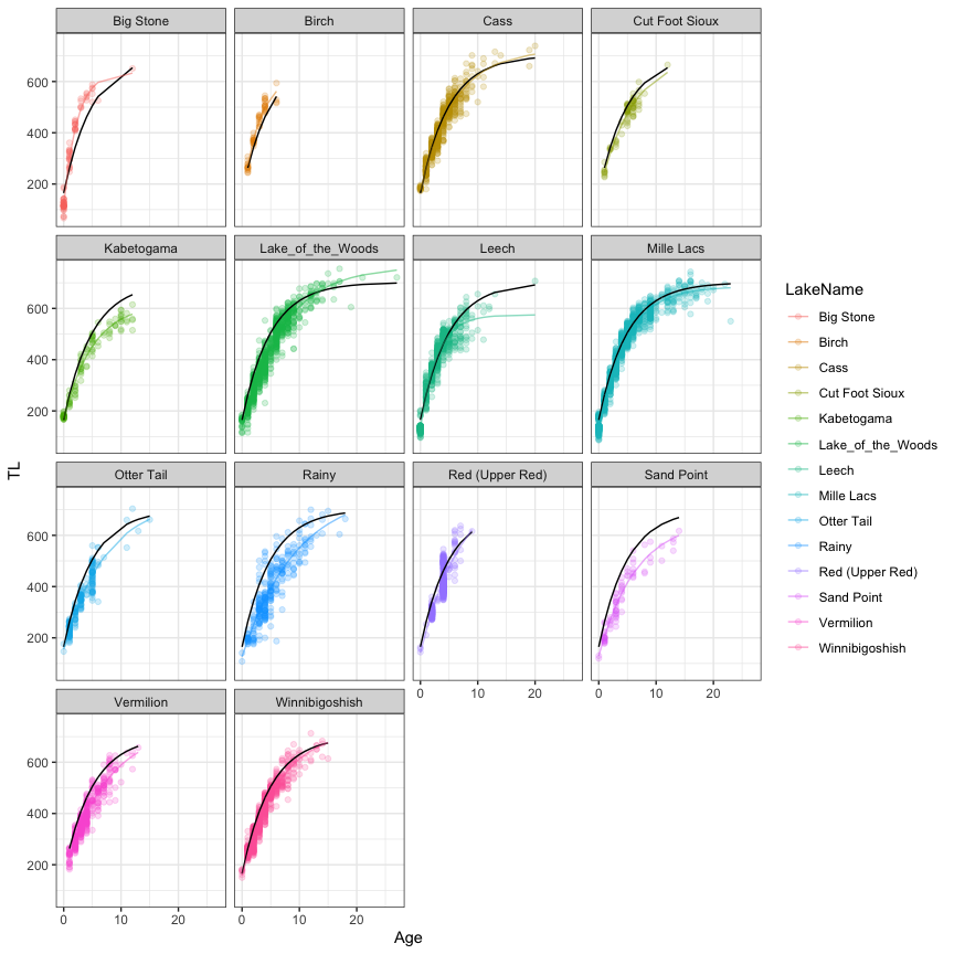
Note that we could smooth the lines by calculating predicted values on a new data frame by specifying regular intervals in age using the expand.grid function as illustrated in the GLMM case study. The parameters estimates at the lake level could be obtained with the coef function:
coef(mod.nlme)
                      Linf         k         t0
Big Stone         636.0669 0.4288756 -0.4916049
Birch             625.1030 0.3453633 -0.6424293
Cass              725.1959 0.1693830 -1.6279210
Cut Foot Sioux    704.4610 0.1723542 -1.4999589
Kabetogama        619.7784 0.1979797 -1.5987604
Lake_of_the_Woods 764.5359 0.1386047 -1.4208832
Leech             575.1076 0.3445203 -0.7696058
Mille Lacs        685.2610 0.2071741 -1.0767931
Otter Tail        738.3058 0.1363032 -1.7370665
Rainy             776.8366 0.1059113 -1.6781612
Red (Upper Red)   840.2491 0.1294834 -1.4276757
Sand Point        660.5877 0.1545496 -1.4147556
Vermilion         735.4408 0.1382678 -1.6648340
Winnibigoshish    731.4472 0.1573876 -1.5338316
Finally, different structures of the model could be compared by updating an existing model. Here, an example if we try to simplify the random component of the model:
#comparing model for the random component
mod.LKT = mod.nlme
mod.LK = update(mod.LKT,random = Linf + k ~1|LakeName)
anova(mod.LK,mod.LKT)
        Model df      AIC      BIC    logLik   Test  L.Ratio p-value
mod.LK      1  7 62056.94 62104.11 -31021.47
mod.LKT     2 10 61718.82 61786.20 -30849.41 1 vs 2 344.1205  <.0001
We confirm that we need a random effect for all parameters. We could also try to include predictors in the fixed effect. Be careful, however, to include the right starting parameter values. See the book of Pinheiro and Bates (2000) for detailed examples.
References
Allegue, H., Y. G. Araya-Ajoy, N. J. Dingemanse, N. A. Dochtermann, L. Z. Garamszegi, S. Nakagawa, D. Réale, H. Schielzeth, and D. F. Westneat. 2017. Statistical Quantification of Individual Differences (SQuID): an educational and statistical tool for understanding multilevel phenotypic data in linear mixed models. Methods in Ecology and Evolution 8:257-267.
Bolker, B. 2009. Learning hierarchical models: advice for the rest of us. Ecological Applications 19:588-592.
Dingemanse, N. J., and N. A. Dochtermann. 2013. Quantifying individual variation in behaviour: mixed-effect modelling approaches. Journal of Animal Ecology 82:39-54.
Faraway, J. 2006. Extending the linear models with R. Chapman and Hall, Boca Raton, Floride.
Gelman, A., and J. Hill. 2006. Data analysis using regression and multilevel / hierarchical models. Cambridge University Press, Cambridge, New York.
Harrison, X. A., L. Donaldson, M. E. Correa-Cano, J. Evans, D. N. Fisher, C. E. D. Goodwin, B. S. Robinson, D. J. Hodgson, and R. Inger. 2018. A brief introduction to mixed effects modelling and multi-model inference in ecology. Peerj 6:e4794.
Honsey, A. E., D. F. Staples, and P. A. Venturelli. 2017. Accurate estimates of age at maturity from the growth trajectories of fishes and other ectotherms. Ecological Applications 27:182-192.
Johnson, P. C. D. 2014. Extension of Nakagawa & Schielzeth’s R2GLMM to random slopes models. Methods in Ecology and Evolution 5:944-946.
Nakagawa, S., P. C. D. Johnson, and H. Schielzeth. 2017. The coefficient of determination R2 and intra-class correlation coefficient from generalized linear mixed-effects models revisited and expanded. Journal of the Royal Society Interface 14:20170213.
Nakagawa, S., and H. Schielzeth. 2013. A general and simple method for obtaining R2 from generalized linear mixed-effects models. Methods in Ecology and Evolution 4:133-142.
Pépino, M., P. Magnan, and R. Proulx. 2018. Field evidence for a rapid adaptive plastic response in morphology and growth of littoral and pelagic brook charr: A reciprocal transplant experiment. Functional Ecology 32:161-170.
Pépino, M., M. A. Rodríguez, and P. Magnan. 2016. Assessing the detectability of road crossing effects in streams: mark–recapture sampling designs under complex fish movement behaviours. Journal of Applied Ecology 53:1831-1841.
Pinheiro, J. C., and D. M. Bates. 2000. Mixed-effects models in S and S-plus. Springer, New York.
Rainville, V., A. Dupuch, M. Pépino, and P. Magnan. 2022. Intraspecific competition and temperature drive habitat-based resource polymorphism in brook charr, Salvelinus fontinalis. Evolutionary Ecology 36:967-986.
Reyjol, Y., M. A. Rodriguez, N. Dubuc, P. Magnan, and R. Fortin. 2008. Among- and within-tributary responses of riverine fish assemblages to habitat features. Canadian Journal of Fisheries and Aquatic Sciences 65:1379-1392.
Schielzeth, H., N. J. Dingemanse, S. Nakagawa, D. F. Westneat, H. Allegue, C. Teplitsky, D. Réale, N. A. Dochtermann, L. Z. Garamszegi, and Y. G. Araya-Ajoy. 2020. Robustness of linear mixed-effects models to violations of distributional assumptions. Methods in Ecology and Evolution 11: 1141– 1152.
Schielzeth, H., and S. Nakagawa. 2013. Nested by design: model fitting and interpretation in a mixed model era. Methods in Ecology and Evolution 4:14-24.
Wagner, T., D. B. Hayes, and M. T. Bremigan. 2006. Accounting for multilevel data structures in fisheries data using mixed models. Fisheries 31:180-187.
Zuur, A. F., and E. N. Ieno. 2016. A protocol for conducting and presenting results of regression-type analyses. Methods in Ecology and Evolution 7:636-645.
Zuur, A. F., E. N. Ieno, N. J. Walker, A. A. Saveliev, and G. M. Smith. 2009. Mixed effects models and extensions in ecology with R. Springer, New York, New York, USA.