Resource selection function
Riwan Leroux
April 2022
- Introduction
- Preparing the database to build RSF
- RSF model
- Quick post-analysis interpretations
- Bibliography
Introduction
Selection analyses framework is suitable to deal with the huge amount of high-frequency data generated by such technological advances (e.g., Resource Selection Function – RSF, Step Selection Function – SSF – Thurfjell et al. 2014, Fieberg et al. 2021, Munden et al. 2021). This analytical framework relies on the comparison between animal’s actual habitat use or real movements and the use or movements of a virtual animal which would randomly move in an environment (Fieberg et al. 2021). By doing so, the virtual animal will encounter ecological features which could be similar or different from what a real animal did (e.g., temperature, biotope, resource density, etc). It is then possible to determine whether or not there is selection of particular features by the followed animal.
Study case
In this study, we focused on lake Ledoux, a small boreal lake where the only fish species is the brook charr (Salvelinus fontinalis), a cold-stenothermic fish. Its main preys are zooplankton in pelagic areas and zoobenthos in littoral areas (Magnan 1988, Bourke et al. 1999). Previous studies suggest that brook charr cannot access epilimnion thus the large shallow basin in the lake Ledoux during summer because of temperature above its lethal threshold of 22°C (Bourke et al. 1996; Bertolo et al. 2011; Goyer et al. 2014). To cope with thermal stress, fish exhibit behavioral thermoregulation which varies according to individuals (Goyer et al. 2014). These individual variations thus could imply individual differences in the feeding strategy. To understand how fish combine their thermoregulation imperatives with the search for resources, we used Resource Selection Analysis (RSF; Boyce & Macdonald 1999; Fieberg et al 2021)
To find the databases needed to the execution of this workshop, please go to :
https://github.com/RiwanLeroux/Numerilab.git
First, lets visualize how, in our study case, a fish moved during 4h in summer 2018 in the lake Ledoux. The ultimate goal of this kind of analysis is to understand whether or not an animal is selecting some environmental variables (e.g. zooplankton, distance to littoral areas, …).
#Import Fish database
load("Fish72.Rdata")
fish<-Fish72; rm(Fish72)

#Import the raster layer of the lake to plot the fish locations on the map
load("Bathymetry_Ledoux.Rdata")

#Look at the fish data frame structure
head(fish)
##                 posix_est        X        Y    Depth   Name burst
## 27993 2018-08-06 12:00:10 1173.186 884.1521 4.662200 Fish72     1
## 27994 2018-08-06 12:00:23 1169.096 883.1159 4.662200 Fish72     1
## 27995 2018-08-06 12:00:36 1165.661 882.2736 4.662200 Fish72     1
## 27996 2018-08-06 12:00:49 1163.142 881.3348 4.740966 Fish72     1
## 27997 2018-08-06 12:01:14 1158.561 879.4407 4.889798 Fish72     1
## 27998 2018-08-06 12:01:36 1155.120 878.0975 5.036059 Fish72     1
#plot the raster
image(ledoux_depth,col=palette,ylim=c(780,1150),main="The 596 locations of the Fish recorded in 4h")

#add the fish locations on the map
points(fish$X,fish$Y,pch=16,cex=0.7)
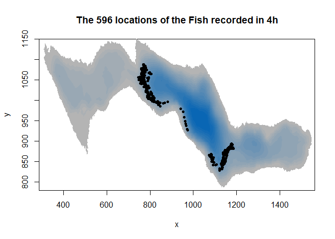
Note that our fish is represented in 2D but moves in 3D. The third dimension is not yet implemented in packages dealing with resource selection function, but lets see what could be done later.
Basically, there are two approaches : Resource or Step Selection Analysis. The first use minimum convex hull to sample points to mimic random location and the second build random steps for each steps the animal make.
Step selection function integrating movement parameters such as step length and turning angles is comparing each observed step from a trajectory with associated simulated steps. Thus, measurements of habitat features must have finer resolution than the average step length to make SSF relevant.
#plot the raster
image(ledoux_depth,col=palette,ylim=c(780,1150),main="Step comparison")

#add the observed steps on the map (length plus angle)
lines(fish$X[c(1:300,400,500,590)],fish$Y[c(1:300,400,500,590)],lty=4)
lines(fish$X[c(300,400)],fish$Y[c(300,400)],lwd=2)
lines(fish$X[c(400,500)],fish$Y[c(400,500)],lwd=2)


#add simulated steps on the map
lines(c(fish$X[300],800),c(fish$Y[300],1050),col="red",lwd=1.5)
lines(c(fish$X[300],840),c(fish$Y[300],970),col="red",lwd=1.5)
lines(c(fish$X[300],950),c(fish$Y[300],1025),col="red",lwd=1.5)

lines(c(fish$X[400],750),c(fish$Y[400],1050),col="forestgreen",lwd=1.5)
lines(c(fish$X[400],700),c(fish$Y[400],1070),col="forestgreen",lwd=1.5)
lines(c(fish$X[400],790),c(fish$Y[400],1055),col="forestgreen",lwd=1.5)
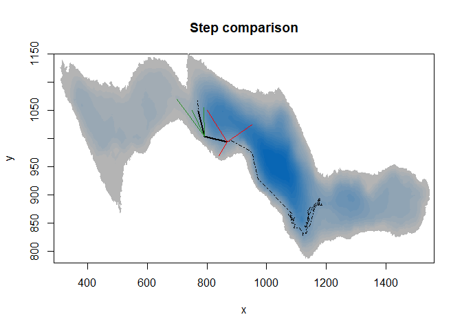 Here SSF would compare each observed black step with corresponding simulated steps. If we considered one-minute step, simulated and observed steps would end really close to each other, with too small differences in environment variables values.
RSF has been privileged over SSF because of the high-frequency acquisition of fish positions. We do not want to reduce much our temporal resolution that SSF required due to our resource sampling resolution
Here we make a mix by building simulated trajectories instead of steps. It enables to better take into account the behavior of the fish who can go at any place suitable for him in the lake but maximize probable response since our resolution remains fine. To build simulated trajectories, we need to have an observed one and randomize it.
Demanding computing time
Make all these validations, for each animal you follow, require a huge amount of data so a huge amount of time. In my study, we have 194 observed trajectories to test. The computation time being too cumbersome to be handled by a personal computer (several months), all these first steps were done with parallel operations (foreach loops;foreach and doParallel packages; see previous Numerilab) on a multicore computer (Titan S599 with 20 cores (+40 Threads) and 96GB of RAM - Titan Computers). Overall, it took three weeks to achieve all the 970,000 simulated trajectories by this approach.
Preparing the database to build RSF
The observed trajectory
To transform our locations into a trajectory, we will use the adehabitatLT package written by Clément Calange (2020). We have an ideal location distribution, with no aberrant location but be aware! If some locations fell outside the lake for example, they have to be removed from the database.
# The function as.ltraj enable us to transform a matrix with time and locations into a succession of steps, with length of the step, the angle between a step and the previous one, the duration of the step etc.

#NB: when we have several fish or periods sampled, this function allows to deal with it by specifying the name of each individuals and the burst (i.e. a succesion of relocation for a specific animal at a specific date). It will result in a list containing all the calculated trajectories.

track_fish=as.ltraj(fish[,c("X","Y")],fish$posix_est,id=fish$Name,
                     burst=fish$burst,slsp="missing",proj4string = crs("+proj=aeqd +lat_0=46.802927 +lon_0=-73.277817 +x_0=1000 +y_0=1000 +datum=WGS84 +units=m +no_defs"))

#lets see what we have. Here, we have one fish tracked during four hours, we have just one burst so one element in the list.
head(track_fish[[1]])
##              x        y                date        dx         dy     dist dt
## 27993 1173.186 884.1521 2018-08-06 12:00:10 -4.090113 -1.0361572 4.219319 13
## 27994 1169.096 883.1159 2018-08-06 12:00:23 -3.434362 -0.8422838 3.536140 13
## 27995 1165.661 882.2736 2018-08-06 12:00:36 -2.519391 -0.9387708 2.688609 13
## 27996 1163.142 881.3348 2018-08-06 12:00:49 -4.581407 -1.8941690 4.957536 25
## 27997 1158.561 879.4407 2018-08-06 12:01:14 -3.440211 -1.3431737 3.693124 22
## 27998 1155.120 878.0975 2018-08-06 12:01:36 -2.465305 -0.3790476 2.494274 11
##             R2n abs.angle   rel.angle
## 27993   0.00000 -2.893480          NA
## 27994  17.80265 -2.901088 -0.00760747
## 27995  60.14627 -2.784912  0.11617599
## 27996 108.81593 -2.749548  0.03536373
## 27997 236.09573 -2.769360 -0.01981231
## 27998 363.01937 -2.989034 -0.21967413
To avoid biases and since we do not want to make integrated step selection analysis (iSSA), we have to homogenize the time-step. We set the time-step to one minute and interpolate the location of fish to have the location of fish at each minute. It also has the advantage to reduce the database and make analysis faster by keeping a relatively high temporal resolution.
#The function redisltraj enables us to homogenize each step to one-minute steps by specifying the step duration in seconds. It will just recalculate the locations of each steps by interpolation.

fixed_track <- redisltraj(track_fish, 60, type="time")

head(fixed_track[[1]])
##          x        y                date         dx         dy      dist dt
## 1 1173.186 884.1521 2018-08-06 12:00:10 -13.892248  -4.408314 14.574903 60
## 2 1159.294 879.7437 2018-08-06 12:01:10 -10.792783  -2.036087 10.983161 60
## 3 1148.501 877.7077 2018-08-06 12:02:10  -7.391698  -4.630913  8.722532 60
## 4 1141.109 873.0767 2018-08-06 12:03:10  -3.540374  -4.736066  5.913084 60
## 5 1137.569 868.3407 2018-08-06 12:04:10   2.804164 -10.162361 10.542149 60
## 6 1140.373 858.1783 2018-08-06 12:05:10  -3.327717  -8.881346  9.484303 60
##         R2n abs.angle  rel.angle
## 1    0.0000 -2.834321         NA
## 2  212.4278 -2.955131 -0.1208105
## 3  650.8811 -2.581914  0.3732175
## 4 1151.5791 -2.212718  0.3691962
## 5 1518.5778 -1.301560  0.9111579
## 6 1751.3242 -1.929292 -0.6277319
Lets plot it !
#plot the background bathymetry map, with a little zoom in the area it used
image(ledoux_depth,col=palette,ylim=c(800,1100),xlim=c(700,1200),main="Raw location vs. Fixed track")

#add the locations of the fish
points(fish$X,fish$Y,pch=16,cex=0.7)

#add the calculated trajectory of the tracked fish
lines(fixed_track[[1]]$x,fixed_track[[1]]$y,col="salmon",lwd=1.5)
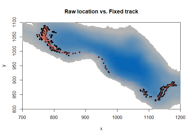
Thus, we have our observed trajectory. Now, we want to simulate trajectories by a randomization of the steps made by the fish. But we want to match the capacity of the individual to cope with the thermal restrains it experiences. And we don’t want him out of the lake.
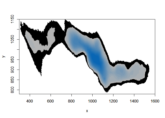
Adding a constraint function
Checking for the minimum depth the fish moved to to have an restrained area where random fish will also be able to move
# Set the minimum depth the fish is able to go
lim_depth=min(fish$Depth,na.rm=T)
print(lim_depth)
## [1] 2.352525
# Create a raster containing only areas of the lake with minimum depth.

# To do so, I inelegantly transform the bathymetry raster into a data frame.
map_temp=as.data.frame(ledoux_depth, row.names=NULL, optional=FALSE, xy=TRUE,
                     na.rm=FALSE, long=FALSE)

# Then I select only the locations of the lake where the lake is deep enough to welcome the observed fish
map_temp=map_temp[which(map_temp$layer>=lim_depth),]

# I create an empty raster with the dimension of the lake original raster
 e <- extent(c(min(map_temp$x),max(map_temp$x),min(map_temp$y),max(map_temp$y)))
  ncellx=(e[2]-e[1])
  ncelly=(e[4]-e[3])
  empty_r<- raster(e, ncol=ncellx, nrow=ncelly)

# Finally I integrate the selected locations into the empty raster
r <- rasterize(map_temp[, 1:2], empty_r, map_temp[,3], fun=mean)

# I built a constraint function which must have SpatialPixelsDataFrame object so we convert the raster
map <- as(r, "SpatialPixelsDataFrame")
crs(map)<-NA

# Here the area in the lake we will let our simulated trajectories go, depending on the depth distribution of the observed fish
image(ledoux_depth,col="black",ylim=c(780,1150),xlim=c(300,1600))
par(new=T)
image(r,ylim=c(780,1150),col=palette,xlim=c(300,1600))
Then we can build a function that will suppress all simulated trajectory that felt outside the defined area
#constraint function which suppress the location if coordinates of a simulated trajectory (x) fell outside of the constrained area (par). This constraint function is one of the arguments integrated to the function simulating trajectories.

consfun <- function(x, par){
  coordinates(x) <- x[,1:2]
  ov <- over(x, geometry(par))
  return(all(!is.na(ov)))
}
Launching the creation of simulated trajectories
First, we create a model, specifying whether or not we want randomized angles or step length and if we force the simulated trajectories to start at the beginning of the observed trajectory. We also have to specify the number of iteration we want to make.
  mo <- NMs.randomCRW(na.omit(fixed_track), rangles=TRUE, rdist=TRUE,
                      constraint.func=consfun,
                      constraint.par = map, nrep=9,fixedStart=TRUE)
Then we have to run the model
Simulated_tracks=testNM(mo)
Lets look at our simulated trajectories
# Transform the list of trajectories into a data frame, adding a column "no" for the trajectory id; 1 being the observed one, and 2 to 10, the 9 simulations
no=1
RSF_database=cbind(fixed_track[[1]][,c(1,2)],no)
for (i in 1:9){
no=i+1
RSF_database=rbind(RSF_database,cbind(Simulated_tracks[[1]][[i]][,c(1,2)],no))
}
# A color vector to have the observed trajectory in color and simulated ones in grey.
couleurs=c("salmon",gray.colors(9, start = 0.3, end = 0.9, gamma = 2.2, rev = FALSE))
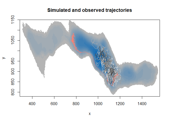
# plot the map
image(ledoux_depth,col=palette,ylim=c(780,1150),main="Simulated and observed trajectories")
#add all trajectory lines
for (i in 10:1){
temp=subset(RSF_database,no==i)
lines(temp$x,temp$y,col=couleurs[i])
}
3D innovation
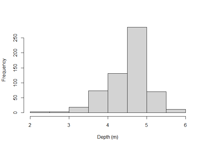
Now, to associate accurate zooplankton data, we have to know in which layer our simulated fish are. To do so, we randomly assign a depth for each random location, picked from the real fish distribution.
• Depth distribution of the fish
distri_depth=fish$Depth
hist(distri_depth,main="",xlab="Depth (m)")
• Recalculation of real depths for the observed trajectory Basically, depth for the “one-minute step” observed trajectory were interpolate from the depth measurements at the original locations framing the step locations
##Lets pass quickly on the recalculation of real depths for the observed trajectory

fixed_track[[1]]$depth=NA

#for loop to assign a depth to each relocation in the observed trajectory
for (i in 1:nrow(fixed_track[[1]])){

  # the time at the relocation i
  time_stamp=as.numeric(substr(fixed_track[[1]]$date[i],12,13))*3600+
                  as.numeric(substr(fixed_track[[1]]$date[i],15,16))*60+
                  as.numeric(substr(fixed_track[[1]]$date[i],18,19))

  # Gathering time for all depth measurements
  time_table=as.numeric(substr(fish[,"posix_est"],12,13))*3600+
                  as.numeric(substr(fish[,"posix_est"],15,16))*60+
                  as.numeric(substr(fish[,"posix_est"],18,19))

  # Selecting the depth where the time of measurement was the closest to the time of the relocation i
  ind_timing1=which(abs(time_stamp-time_table)==min(abs(time_stamp-time_table),na.rm=T))
          print(c(i,length(ind_timing1)))

  # If both previous and next closest depth measurement are equally distant, we average the depth between the two to have the depth at relocation i
   if(length(ind_timing1)==2){
                fixed_track[[1]]$depth[i]=mean(fish[,"Depth"][ind_timing1])
   }

  # If we have only one closest depth measurement
   if(length(ind_timing1)==1){

  # If the closest depth measurement is after the time of relocation i, we take this measurement and the one before and then make a linear interpolation to retrieve the depth at relocation i
    if(time_stamp-time_table[ind_timing1]<0){
      ind_timing2=ind_timing1-1
      time=time_table[ind_timing1]-time_table[ind_timing2]
      depth_var=fish[ind_timing1,"Depth"]-fish[ind_timing2,"Depth"]
      depth_inter=(time_stamp-time_table[ind_timing2])*(depth_var/time)+fish[ind_timing2,"Depth"]
      fixed_track[[1]]$depth[i]=depth_inter
    }

  # If the closest depth measurement is before the time of relocation i, we take this measurement and the one after and then make a linear interpolation to retrieve the depth at relocation i
    if(time_stamp-time_table[ind_timing1]>0){
      ind_timing2=ind_timing1+1
      time=time_table[ind_timing2]-time_table[ind_timing1]
      depth_var=fish[ind_timing2,"Depth"]-fish[ind_timing1,"Depth"]
      depth_inter=(time_stamp-time_table[ind_timing1])*(depth_var/time)+fish[ind_timing1,"Depth"]
      fixed_track[[1]]$depth[i]=depth_inter

    }
  # If the closest depth measurement is at the exact time of relocation i, we directly take this measurement to assign the depth at relocation i
    if(time_stamp-time_table[ind_timing1]==0){
      fixed_track[[1]]$depth[i]=fish[ind_timing1,"Depth"]
    }
  }
}
• Assignment of depth to simulated trajectories
To assign depth to simulated trajectories, it is necessary to control for the depth of the water column to be sure our random fish is not in the ground. Then, just sample randomly the distribution.
  # Create a column to inform the depth of the water column at each simulated location
RSF_database$max_depth=NA

  # Use the extract function of the raster package to retrieve the water column depth for each simulated locations
RSF_database$max_depth=extract(ledoux_depth,RSF_database[,c(1:2)])

  # Empty vector
depth_random=NA
  #for loop where we paste each depth randomized sampling with the vector
  for (i in which(RSF_database$no!=1)){
    depth_random=c(depth_random,sample(distri_depth[which(distri_depth<=RSF_database$max_depth[i])],1))
  }
  #Then, in the database regrouping all observed and simulated trajectories, we add the depth column

RSF_database$depth=c(fixed_track[[1]]$depth,depth_random[-1])

#Lets see how our depth distribution behaved

ggplot(RSF_database,aes(x=depth))+
  geom_histogram(position="dodge",bins=15)+
  facet_wrap(~no)
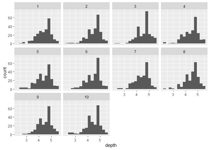
Histograms of depth distribution for each trajectory
Assign values for the tested variables
Once we have 3D locations, we can add the corresponding values of the variables we want to test. Here, we could for example add the value of biovolume of zooplankton larger than 1mm encoutered at each location. It is the same principle than when extracting the maximum depth from a raster but we have as many raster as we have different depth levels (every meters).
  # Create a vector of depth breaks
depth_vector=seq(-0.5,16.5,1)

  # Load the zooplankton database
load("large_Z.Rdata")

  # Create the column with future zooplankton concentrations
RSF_database$LZ=NA

  # Create empty raster to create zooplankton raster to be extracted for each depth layer.
e <- extent(ledoux_depth)
  #Wished horizontal resolution : 5m per 5m
ncellx=(e[2]-e[1])/5
ncelly=(e[4]-e[3])/5
r<- raster(e, ncol=ncellx, nrow=ncelly)

  # For loop to assign zooplankton concentrations at both simulated and observed locations for each depth layer
for (prof in 1:(length(depth_vector)-1)){

  # Subset of the trajectories database with only locations in the right depth layer
  temp=RSF_database[which(RSF_database$depth>=depth_vector[prof]&RSF_database$depth<depth_vector[prof+1]),]

  # If we have any locations here
    if(nrow(temp)>0){

  # Select the zooplankton measurements for the corresponding depth layer
      tempZ=Large_zooplankton[which(Large_zooplankton$Depth==(depth_vector[prof]+0.5)),c("X","Y","Predicted")]

  # Transform it into a raster
      temp_rast_LZ <- rasterize(tempZ[, 1:2], r, tempZ[,3], fun=mean)

  # Extract the zooplankton concentrations for all the locations in this depth layer
      RSF_database$LZ[which(RSF_database$depth>=depth_vector[prof]&RSF_database$depth<depth_vector[prof+1])]=extract(temp_rast_LZ,RSF_database[which(RSF_database$depth>=depth_vector[prof]&RSF_database$depth<depth_vector[prof+1]),c(1,2)])
    }
}

head(RSF_database)
##          x        y no max_depth    depth        LZ
## 1 1173.186 884.1521  1  6.024511 4.662200 0.7207559
## 2 1159.294 879.7437  1  6.263787 4.865985 0.7048485
## 3 1148.501 877.7077  1  7.330539 5.414200 0.6943779
## 4 1141.109 873.0767  1  7.961336 5.494100 0.7068840
## 5 1137.569 868.3407  1  8.414603 5.564600 0.4528299
## 6 1140.373 858.1783  1  7.483882 5.275326 0.7034004
Once all variables are attached to the RSF database, we are almost done ! We still have to weight the available points compared to the used one (for explanations, see Fithian & Hastie 2013 or Fieberg et al 2021). The next step is to run a conditional logistic regression with the database to finally have our coefficients of seletion.
RSF_database$weight=ifelse(RSF_database$no==1,1,5000)
RSF model
So RSF is just conditional logistic regression, with just some subtleties…
  #To conditional regression, we need a TRUE / FALSE variable. Here, only the no 1 trajectory is TRUE since it is the observed one
RSF_database$case=RSF_database$no==1

  # Scale the variables
RSF_database$LZ=scale(RSF_database$LZ)
RSF_database$max_depth=scale(RSF_database$max_depth)

  # Write the regression model
RSF_model= glm(case ~ max_depth + LZ,data = RSF_database,weight=weight, family = binomial(link = "logit"))

summary (RSF_model)
##
## Call:
## glm(formula = case ~ max_depth + LZ, family = binomial(link = "logit"),
##     data = RSF_database, weights = weight)
##
## Deviance Residuals:
##     Min       1Q   Median       3Q      Max
## -2.2934  -0.4099  -0.1174  -0.0335   4.7826
##
## Coefficients:
##             Estimate Std. Error z value Pr(>|z|)
## (Intercept) -12.6212     0.2119 -59.567  < 2e-16 ***
## max_depth    -2.7535     0.1795 -15.337  < 2e-16 ***
## LZ           -0.5705     0.0824  -6.924  4.4e-12 ***
## ---
## Signif. codes:  0 '***' 0.001 '**' 0.01 '*' 0.05 '.' 0.1 ' ' 1
##
## (Dispersion parameter for binomial family taken to be 1)
##
##     Null deviance: 5508.0  on 2359  degrees of freedom
## Residual deviance: 4948.9  on 2357  degrees of freedom
##   (40 observations effacées parce que manquantes)
## AIC: 4954.9
##
## Number of Fisher Scoring iterations: 8
Both deep water column and zooplankton concentration are negatively selected. Zooplankton avoided? To be continued… … Once we have the coefficient, we can calculate the Resource Selection Strengh (RSS) as RSS=exp(coeff). RSS is the probability that a fish will be found in an area with RSS times the variable tested when the value of this variable increased by one unit.
RSS_zoo=exp(RSF_model$coefficients[3])
paste0("RSS = ",round(RSS_zoo,3))
## [1] "RSS = 0.565"
However, careful to the number of simulated trajectories necessary and to the significance of the model !
These parts require lots of computing time (several days for just one fish) so here is some already made validations.
Control how many simulated trajectories are needed
  # Here a database containing regression estimates calculated 10 times with various number of simulated trajectories for our fish
N_Simul=read.csv("S4_base.csv")
N_Simul_Z=N_Simul[which(N_Simul$param=="Large zooplankton"),]


ggplot(N_Simul_Z, aes(y=coeff,group=N_random_tracks))+
  geom_boxplot(outlier.shape = NA)+
  theme_bw()+
  xlab("Number of simulated trajectories")+
  scale_x_continuous(breaks=c(seq(-0.4,0.4,0.8/6)),
                   labels=as.character(seq(0,300,50)))+
  geom_vline(xintercept=0,lty=2)+
  theme(axis.title.x = element_text(size=14),axis.text.x = element_text(size=14),axis.text.y = element_text(size=14))+
  theme(legend.position = "None")+
  ylab(paste0("RSF estimate"))
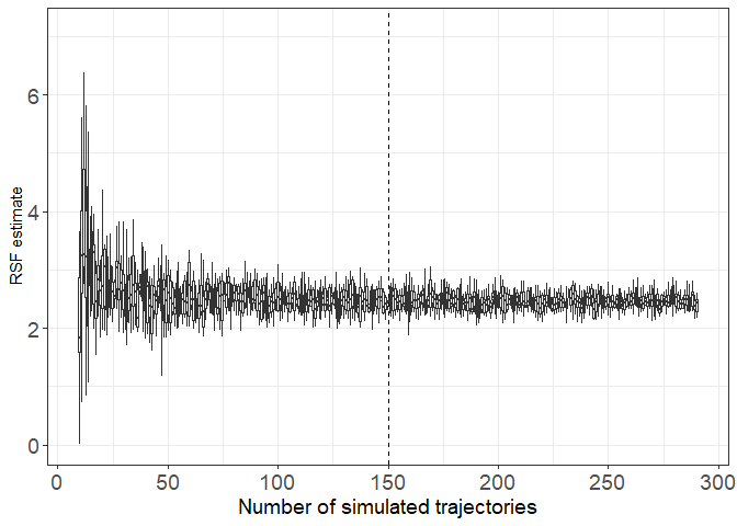
Here we are noticing a large variability of estimates when less than 50 simulated trajectories are build to calculate the coefficient of the logistic regression. To be conservative, I decided to keep 150 simulated trajectories to be sure we have a stable coefficient estimation.
Control for the p-value
Since our regression is based on thousands of points, the sample size could induced automatic significance of the p-value. To avoid this bias, we built the distribution of estimates under the null hypothesis. It means that the regression coefficient we calculate must be greater or lower from at least 95% of estimates which would be calculated from a comparison of a simulated trajectory with 150 other simulated trajectories.
  # Import database where we calculated 500 times the regression based one simulated trajectory and 150 other simulated trajectory
H0_500=read.csv("HO_500.csv")

    # Import database where we calculated a various number of times the regression based one simulated trajectory and 150 other simulated trajectory
H0_data= read.csv("S5DB.csv",row.names=1)

ggplot(H0_500, aes(x=RSF_estimate))+
  geom_histogram(fill="gray80",colour="gray50",bins=18,aes(y=(..count../sum(..count..)) * 100))+
  theme_bw()+
  geom_vline(xintercept = quantile(H0_500$RSF_estimate,c(0.025,0.975)),lty=2)+
  xlab("RSF estimate")+
  theme(axis.title.y = element_text(size=14),axis.title.x = element_text(size=14),axis.text.x = element_text(size=14),axis.text.y = element_text(size=14))+
  theme(legend.position = "None")+
  ylab(paste0("Percentage of occurrence (%)"))
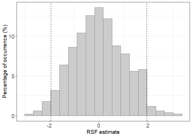
When we calculate the RSF for the fish, the coefficient must be outside the range [-2;2] to be considered different from 0 (i.e. to show active selection or avoidance). Here, the distribution is drawn after repeating 500 H0 RSF. But this number has to be previously assessed to be sure it is sufficient to build the H0 distribution.
  ggplot(H0_data, aes(y=inf,x=N_H0_RSF))+
  geom_smooth(col="gray50")+


  geom_smooth(aes(y=sup,x=N_H0_RSF),col="gray50")+
  geom_point()+
  geom_point(aes(y=sup,x=N_H0_RSF))+
  theme_bw()+
  geom_vline(xintercept = 500,lty=2)+
  xlab("Number of RSF iterations")+
  theme(axis.title.y = element_text(size=14),axis.title.x = element_text(size=14),axis.text.x = element_text(size=14),axis.text.y = element_text(size=14))+
  theme(legend.position = "None")+
  ylab(paste0("Boundaries of the 5% confidence interval of RSF estimates"))
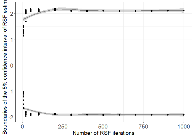
We see that with more than 400 iterations, the 95% confidence interval is stable. We chose 500 iterations to be conservative.
Quick post-analysis interpretations
Let’s see some actual results, in terms of selection occurrences, intensities and interactions. (Leroux et al. in prep)
Bibliography
Bertolo, A., Pépino, M., Adams, J., & Magnan, P. (2011). Behavioural thermoregulatory tactics in lacustrine brook charr, Salvelinus fontinalis. PLoS One, 6(4), e18603.
Bourke, P., Magnan, P., & Rodriguez, M. A. (1996). Diel locomotor activity of brook charr, as determined by radiotelemetry. Journal of Fish Biology, 49(6), 1174-1185.
Bourke, P., Magnan, P., & Rodríguez, M. A. (1999). Phenotypic responses of lacustrine brook charr in relation to the intensity of interspecific competition. Evolutionary Ecology, 13(1), 19-31.
Boyce, M. S., & McDonald, L. L. (1999). Relating populations to habitats using resource selection functions. Trends in ecology & evolution, 14(7), 268-272.
Calenge, C. (2011). Analysis of animal movements in R: the adehabitatLT package. R Foundation for Statistical Computing, Vienna.
Fieberg, J., Signer, J., Smith, B., & Avgar, T. (2021). A ‘How to’guide for interpreting parameters in habitat‐selection analyses. Journal of Animal Ecology, 90(5), 1027-1043.
Fithian, W., & Hastie, T. (2013). Finite-sample equivalence in statistical models for presence-only data. The annals of applied statistics, 7(4), 1917.
Goyer, K., Bertolo, A., Pépino, M., & Magnan, P. (2014). Effects of lake warming on behavioural thermoregulatory tactics in a cold-water stenothermic fish. PLoS One, 9(3), e92514.
Magnan, P. (1988). Interactions between brook charr, Salvelinus fontinalis, and nonsalmonid species: ecological shift, morphological shift, and their impact on zooplankton communities. Canadian Journal of Fisheries and Aquatic Sciences, 45(6), 999-1009.
Munden, R., Börger, L., Wilson, R. P., Redcliffe, J., Brown, R., Garel, M., & Potts, J. R. (2021). Why did the animal turn? Time‐varying step selection analysis for inference between observed turning‐points in high frequency data. Methods in Ecology and Evolution, 12(5), 921-932.
Thurfjell, H., Ciuti, S., & Boyce, M. S. (2014). Applications of step-selection functions in ecology and conservation. Movement ecology, 2(1), 1-12.