Interactive R applications with Shiny
Charles Martin
April 2021
- Introduction
- A first application
- A whole gamut of controls
- Output elements available
- Making your application more efficient
- Information sharing rules inside a Shiny app
- How to publish a Shiny app
- Customizing the interface layout
- Resources
Introduction
Today in this workshop, we will see how create interactive R applications, using the Shiny library. You will learn how to create environments where you readers will be able to interact with your data and models, instead of being offered a static final product.
If you need ideas about how to turn your data into interactive applications, the official Shiny gallery https://shiny.rstudio.com/gallery/ is a very good place to start.
Consequently, this workshop has almost not statistical concepts to learn or understand, but you will need to do a lot of programming.
Before diving into our first Shiny application, it is important to understand how such an application is usually structured. Our code will be separated in two main functions.
A first function will define the interface which the user will be shown (the User Interface or ui function). This interface will take the form of a web page in the user’s web browser (i.e. usually Google Chrome, Apple’s Safari or MS Edge). Hopefully, you will not need to write any HTML, Javascript or CSS to make this work. You will use a meta-language to define what you wish to show the user, and Shiny will translate it into proper HTML code.
Our second important function will define actions to do when the user interacts with your interface, which we call here the server function.
Once both these functions (ui and server) are defined, we will use a single R line to connect the two together into an application object, which can be launched.
At first, such a drastic separation might seem like a useless complication, but separating interface code from server code is a software engineering best practice that has proved its worh for many decades. In many cases, the practice goes even farther, into what is commonly called the MVC (Mode-View-Controller) paradigm, where the application is split in three pieces : database management, user interface and server code. In fact, this kind of seperation was so important for Shiny authors that early versions of the library forced you to put interface and server code into separate files.
A first application
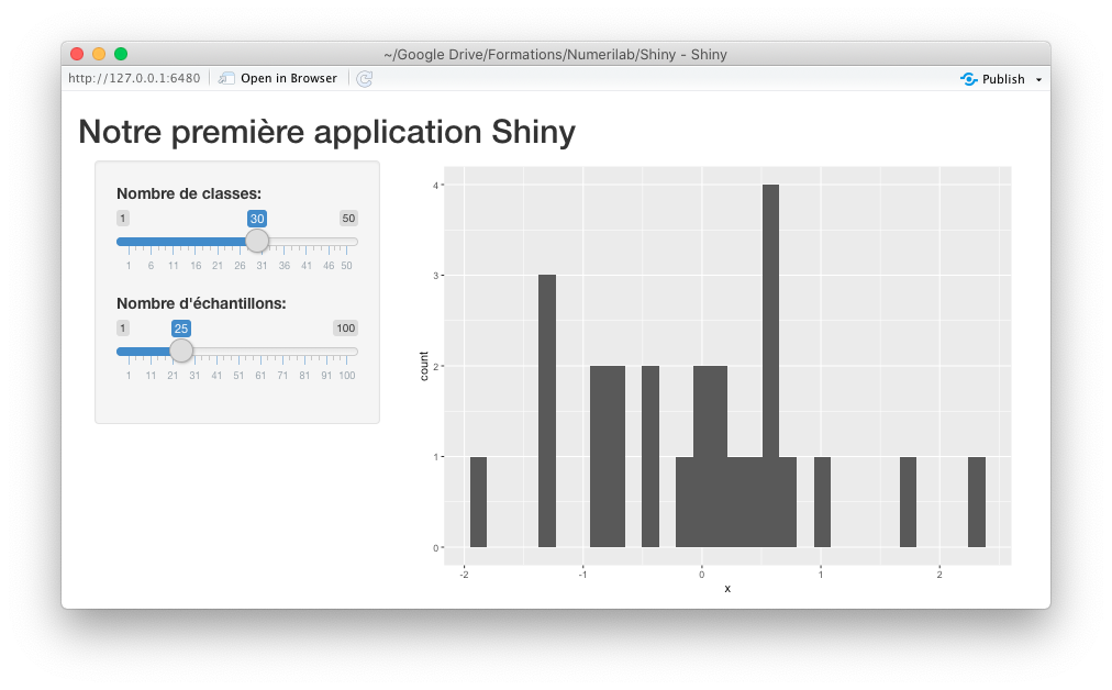
That said, let’s start our first little Shiny application. As a first project, I suggest we do a little interactive histogram viewer, where the user will be allowed to select a sample size to pick from a normal distribution, along with the number of classes the histogram should display.
First, our code needs to activate the Shiny library, and we will also need both ggplot2, dplry and tidyr, as usual.
library(shiny)
library(ggplot2)
library(dplyr)
Attaching package: 'dplyr'
The following objects are masked from 'package:stats':

    filter, lag
The following objects are masked from 'package:base':

    intersect, setdiff, setequal, union
library(tidyr)
Then, we will define the user interface of our application. First, here’s some code to organize the web page a bit :
interface <- fluidPage(
  titlePanel("Notre première application Shiny"),
  sidebarPanel(),
  mainPanel()
)
We are asking R to create an interface containing a title panel, a side bar to contain the necessary controls and a main panel, where we will display our plot.
Now, lot’s modify this code, to add the individual pieces of our interface :
interface <- fluidPage(
  titlePanel("Notre première application Shiny"),
  sidebarPanel(
    sliderInput(
      inputId = "nb_classes",
      label = "Nombre de classes:",
      min = 1,
      max = 50,
      value = 30
    ),
    sliderInput(
      inputId = "nb_echantillons",
      label = "Nombre d'échantillons:",
      min = 1,
      max = 100,
      value = 25
    )
  ),
  mainPanel(
    plotOutput(outputId = "graphique_histogramme")
  )
)
Notice that, for every control, we need to specify an ID, which will allow us to reference this control later on in the server code.
Now that we have defined our user interface, we will need to create a little server to use the user-selected control values to customize our histogram :
serveur <- function(input, output) {

  output$graphique_histogramme <- renderPlot({

    # Bloquer le générateur de nombre aléatoires pour toujours obtenir la même séquence
    set.seed(4847)
    donnees <- data.frame(
      x = rnorm(n = input$nb_echantillons)
    )

    ggplot(donnees, aes(x = x)) +
      geom_histogram(bins = input$nb_classes)

  })

}
Our server function always receives two objects as arguments, named input and output. These arguments are used to, respectively, receive user inputs and display information to her.
Now, we only need to connect all this together into an application object, and run it :
appli <- shinyApp(ui = interface, server = serveur)
runApp(appli)
A whole gamut of controls
Now that we have created our first working application, let’s see what controls we can use to let our user control the app and produce an even more customized graphic.
We will use double sliders to determine the range of X and Y values visible, a single to handle the point size, along with checkboxes to decide which animal groups to display and a radio button to decide which type of smoothing function to add to our plot. Finaly, we’ll display our user a text box to enter the title of our plot.
So, let’s create this new user interface :
interface2 <- fluidPage(

  titlePanel("Deuxième application : les contrôles"),

  sidebarPanel(

    sliderInput("limites_x", "Limites de l'axe des X",min = 0, max = 7, value = c(0, 7)),
    sliderInput("limites_y", "Limites de l'axe des Y",min = 0, max = 25, value = c(0, 25)),
    sliderInput("taille_points", "Taille des points", min=0, max = 10, value = 1),

    radioButtons(
      "type_lissage",
      "Type de lissage",
      choices = list("Régression" = "lm","Loess" = "loess"),
      selected = "lm"
    ),

    textInput("titre", "Titre du graphique", value = "Entrez votre titre ici"),

    checkboxGroupInput(
      "groupes",
      "Quel groupes voulez-vous afficher?",
      choices = list(
        "Herbivores" = "herbi",
        "Carnivores" = "carni",
        "Omnivores" = "omni",
        "Insectivores" = "insecti"
        ),
      selected = c("carni","herbi","omni","insecti")
    )
  ),

  mainPanel(
    plotOutput(outputId = "graphique")
  )

)
And now, we need some server code to explain to our app how to use the values selected by our user to customize our graphic :
serveur2 <- function(input, output) {

  output$graphique <- renderPlot({

    msleep %>%
      filter(vore %in% input$groupes) %>%
      ggplot(aes(x = sleep_rem, y = sleep_total)) +
        geom_point(size = input$taille_points, aes(color = vore)) +
        xlim(input$limites_x) +
        ylim(input$limites_y) +
        geom_smooth(method = input$type_lissage) +
        labs(title = input$titre)
  })
}
You see that, the value of each and every control on the page is usable as a slot from the input object, using the IDs mentioned while building the interface.
appli2 <- shinyApp(ui = interface2, server = serveur2)
runApp(appli2)
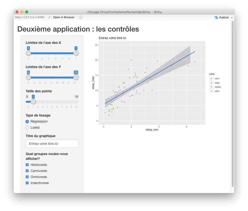
Notice the nuance between radio buttons and checkboxes. The usual convention is that radio buttons are used to select a single option at a time, whereas checkboxes allow you to select many options.
Output elements available
Now that we have seen the many ways to grab user inputs, lets see what are our options to display outputs to her.
As we have seen in the previous two examples, the plotOutput object can be used to display graphics. There are also objets to display tables (tableOutput) as well as text (textOutput).
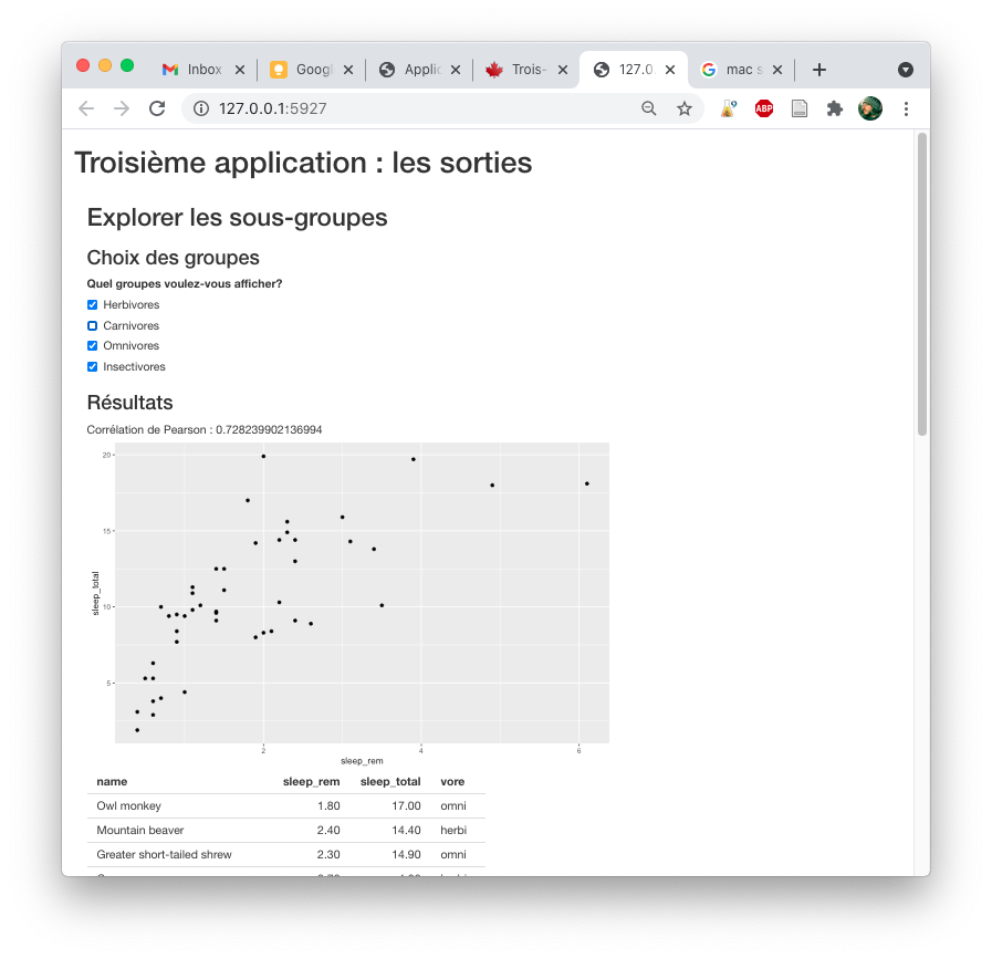
Let’s put all these pieces together to build a third application, in which we’ll allow our user to explore the msleep data set.
You will also see that in this example, I’m using elements named h1, h2, etc., which are used to create titles of different levels in your interface, like you would do in Word.
interface3 <- fluidPage(
  h1("Troisième application : les sorties"),
  mainPanel(
    h2("Explorer les sous-groupes"),

    h3("Choix des groupes"),
    checkboxGroupInput(
      "groupes",
      "Quel groupes voulez-vous afficher?",
      choices = list(
        "Herbivores" = "herbi",
        "Carnivores" = "carni",
        "Omnivores" = "omni",
        "Insectivores" = "insecti"
        ),
      selected = c("carni","herbi","omni","insecti")
    ),

    h3("Résultats"),
    textOutput(outputId = "chiffre_correlation"),
    plotOutput(outputId = "graphique_correlation"),
    tableOutput(outputId = "donnees_correlation")
  )

)
In the corresponding server code, we will simply filter the msleep data set, based on the user choices, and then calculate and display the resulting correlation.
Notice that now, our code has many render functions, one for each output we described in the interface.
serveur3 <- function(input, output) {

  output$graphique_correlation <- renderPlot({
      sous_groupes <- msleep %>% filter(vore %in% input$groupes)
      ggplot(sous_groupes, aes(x = sleep_rem, y = sleep_total)) +
        geom_point()
  })

  output$chiffre_correlation <- renderText({
      sous_groupes <- msleep %>% filter(vore %in% input$groupes) %>%
        select(sleep_rem, sleep_total) %>%
        drop_na
      paste0(
        "Corrélation de Pearson : ",
        cor(sous_groupes$sleep_rem, sous_groupes$sleep_total)
      )
  })

  output$donnees_correlation <- renderTable({
      sous_groupes <- msleep %>%
        filter(vore %in% input$groupes) %>%
        select(name, sleep_rem, sleep_total, vore) %>%
        drop_na
      sous_groupes
  })

}
appli3 <- shinyApp(ui = interface3, server = serveur3)
runApp(appli3)
Making your application more efficient
One thing you might have noticed in the preceeding example is that, the data filtering code is duplicated in many places in the app.
To make this code more efficient, we will need to understand a bit of the inner workings of a Shiny application.
First, you might have noticed that, any time you change the value from a control input, the whole page isn’t reloaded, only the related outputs are. This can happen because, when you launch the application, Shiny explores all your render functions, and creates observers for them, which spy on the inputs they use to see if their value changes.
One way our application could be more efficient here was if every time a control value was changed we built the correct filtered dataset, and then if any associated output could be updated with the new data. It won’t make much of a difference here on dozens of lines, but if you had thousands of lines to filter, or much more complexe and tedious calculations, there would be real gains to be made.
From a maintenance point of view, having the same code duplicated in three places is also a recipe for disaster.
The way to reorganize that code is through what Shiny calls reactive expressions. The expressions are kind of smart functions, which are only executed when the controls they refer to are modified. Once that is done, subsequent calls are much faster because they send you back the cached value, instead of doing the calculations again and again.
Shiny builds for us a kind of dependency graph, where our outputs depend on the reactive expression, and the reactive expression depends on the user controls. If any pieces of the graph are modified, Shiny intelligently updates all the pieces that depend on it, but doesn’t touch any of the other pieces.
serveur3b <- function(input, output) {

  sous_groupes <- reactive({
    msleep %>% filter(vore %in% input$groupes) %>%
      select(sleep_total, sleep_rem, vore, name) %>%
      drop_na

  })

  output$graphique_correlation <- renderPlot({
      ggplot(sous_groupes(), aes(x = sleep_rem, y = sleep_total)) +
        geom_point()
  })

  output$chiffre_correlation <- renderText({
      paste0(
        "Corrélation de Pearson : ",
        cor(sous_groupes()$sleep_rem, sous_groupes()$sleep_total)
      )
  })

  output$donnees_correlation <- renderTable({
      sous_groupes()
  })

}
appli3b <- shinyApp(ui = interface3, server = serveur3b)
runApp(appli3b)
Notice how sous_groupes now needs to be used as an R function, with parenthesis, instead of using it as a normal R object. It is a bit tedious, be allows us to regroup all of our calculations in a single place, and avoid waisting important calculation time.
Information sharing rules inside a Shiny app
In a Shiny app, your code is not a simple script running on your personnal machine anymore. It is a web application, that can be used by many users simultaneously. It is thus important do understand how information is divided inside the app.
There are essentially two levels : global objects, which are shared between all users simultaneously, and session objets, which are private to each user. Objects will belong to a level or the other depending on where they were defined in your code.
In a gist : any object defined outside the server and interface functions are global objects, whereas anything defined inside server and interface functions is user-specific. As of now, we have only played with user-specific objects. Pierre’s point size change on his plot is not supposed to affect Jacques’.
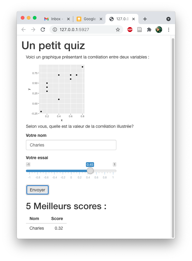
Let’s see a case where users might wish to share some information between them with a little quiz application, where the goal is to guess the correlation between two variables.
In this app, we will not only need an interface and a server function, but also a global data.frame to store the scores from all of our users.
Notice that our data.frame was wrapped in a reactiveValues function. As in our previous app, this wrapping allows Shiny to listen to changes made on this data.frame, which in turn will update all outputs that rely on this data.
At this step, and also outside server and interface function, I prepare the data I’ll use for the correlation per se. I prepare it in the global environment, because it is common to all users. But I don’t wrap it in a reactiveValues function, because these values are fixed.
objets_reactifs <- reactiveValues(
  meilleurs_scores = data.frame(
    Nom = character(),
    Score = numeric()
  )
)

donnees_pour_correlation <- data.frame(
  x = c(0.7, 0.4, 0.4, 0.8, 0.1, 0.2, 0.2, 0.6, 0.2, 0.6),
  y = c(0.7, 0.7, 0.1, 0.9, -0.2, 0.4, 0.3, 0.7, 0.5, 0.6)
)
For the interface, nothing too compliated. I used input and output objects as we have seen before. I use a new function, called p, which adds a paragraph of text in the interface.
Also notice how I control the height and width of the plotOutput object.
interface_quiz <- fluidPage(

  h1("Un petit quiz"),

  mainPanel(

    p("Voici un graphique présentant la corrélation entre deux variables :"),

    plotOutput("graphique_correlation", width = "200px", height = "200px"),

    p("Selon vous, quelle est la valeur de la corrélation illustrée?"),

    textInput("nom", "Votre nom", value = ""),
    sliderInput("essai", "Votre essai", value = 0, min=-1,max=1,step=0.01),
    actionButton("envoyer", label = "Envoyer"),

    h2("5 Meilleurs scores : "),
    tableOutput("tableau_scores")

  )
)
Our server function contains three code blocks.
The first two blocks define what to display in our results table and our correlation plot, using the same strategies we have seen above in other applications.
The third code block defines what to do when the user clicks the Send button. It observes the button, and runs when it is clicked.
At that moment, we calculate the user’s score (the absolute difference between its guess and the actual correlation) and convert that info into a data.frame row.
We then display the results to the user using the notification function.
Finally, we update the best scores table. Notice that for this operation, we use the «- operator, to access the global results table.
Since our results data.frame is a reactive object, its associated output is automatically updated, for every connected user at once.
serveur_quiz <- function(input, output) {

    output$tableau_scores <- renderTable({
      objets_reactifs$meilleurs_scores %>%
      arrange(Score) %>%
      slice(1:5)
  })

  output$graphique_correlation <- renderPlot(
    ggplot(donnees_pour_correlation,aes(x=x,y=y)) +
      geom_point()
  )

  observeEvent(input$envoyer, {

    score = abs(
      input$essai -
        cor(donnees_pour_correlation$x,donnees_pour_correlation$y)
    )

    nouvel_essai <- data.frame(
      Nom = input$nom,
      Score = score
    )


    showNotification(paste0("Vous vous êtes trompé par ",score))

    objets_reactifs$meilleurs_scores <<-
      objets_reactifs$meilleurs_scores %>%
      bind_rows(nouvel_essai)

  })


}
appli_quiz <- shinyApp(ui = interface_quiz, server = serveur_quiz)
runApp(appli_quiz)
Of course, as of now, you are still only playing the quiz alone on your computer. We’ll see in the next section how to publish an app for everyone to use.
How to publish a Shiny app
First of all, it is important to understand that in order to publish a Shiny app, you’ll need a web server to run it. When you launch the runApp command, R starts for you a little web server so that you can test your application. But, as you might have guessed, it is not the correct way to publish an app for everyone to use.
The simplest way to make your application public is to the the http://shinyapps.io service. On Shinyapps.io, you can publish up to 5 applications per user, up to 25 hours of usage time monthly for free. There is also a pricing structure, running between 9$ a month up to 3300$ a year, depending on how many applications and how many running hours you need.
To use ShinyApps.io, the easiest way is to start a new project in RStudio, and choose Shiny Web Application as a project type and put all your code in a file named app.R.
Once your application is ready for primetime, just remove the runApp line (ShinyApps.io will start the app for you) and you are ready to go.
To be begin the publishing process, click the File… Publish… menu item
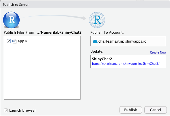
RStudio will ask you to retrive a token on the ShinyApps.io website, proving that your are allowed to publish apps using the specified account.
Once that is done, just hit the Publish button to put your app online. You will see that this process is not instantaneous. It might take several minutes, because ShinyApps.io must create a new R instance for your app, install the relevant packages, upload your content, start your app, etc.
At the end of the publishing process, your app will automatically open in your web browser (probably Google Chrome). As an example, I’ve published the correlation quiz we’ve built above at the address : https://charlesmartin.shinyapps.io/QuizCorrelation/
If you want to update your app, just click again on File… Publish … to replace your old version with the new.
If you have a more technical background, you can also install the open source version of the Shiny Server (https://rstudio.com/products/shiny/shiny-server/) on a Linux-running server to which you already have access.
Customizing the interface layout
The last item on our agenda today is : how to customize our Shiny apps.
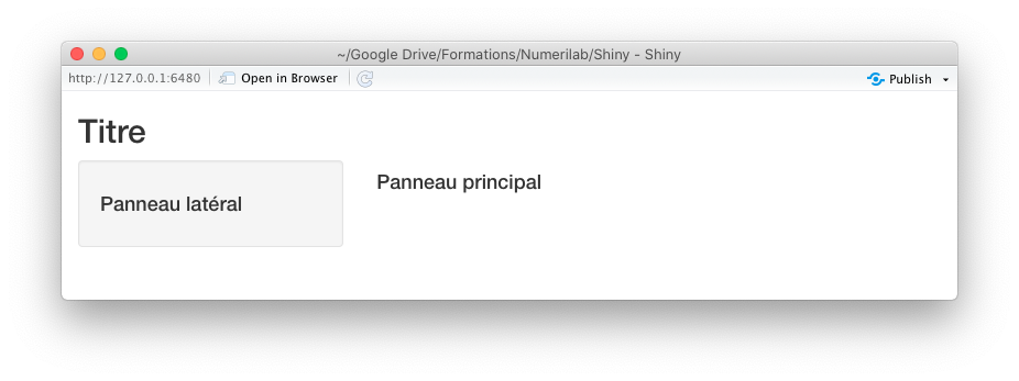
All the above examples used the same layout, which is a sidebarPanel and a mainPanel, as in :
interface_avec_panneau <- fluidPage(

  titlePanel("Titre"),

  sidebarLayout(
    sidebarPanel(
      h4("Panneau latéral")
    ),
    mainPanel(
      h4("Panneau principal")
    )
  )
)
serveur_vide <- function(input, output) {
}
appli <- shinyApp(ui = interface_avec_panneau, server = serveur_vide)
runApp(appli)
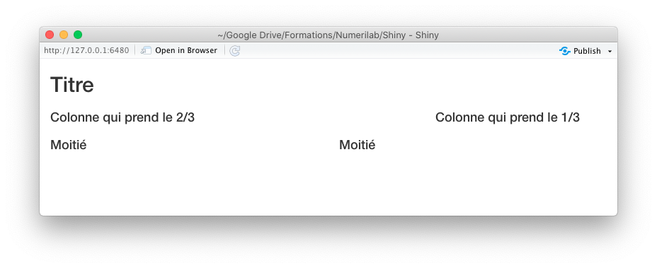
One of the alternative options is to use a grid layout, where every grid row is defined by a fluidRow function, and every cell is defined by a column function. To customize the width of the cell, keep in mind that Shiny expects the columns to sum up to 12 units. For example, to do a 2/3 - 1/3 layout, you must choose 8 and 4 as column widths :
interface_grille <- fluidPage(

  titlePanel("Titre"),

  fluidRow(
    column (8,h4("Colonne qui prend le 2/3")),
    column (4,h4("Colonne qui prend le 1/3"))
  ),
  fluidRow(
    column (6,h4("Moitié")),
    column (6,h4("Moitié"))
  )
)
appli <- shinyApp(ui = interface_grille, server = serveur_vide)
runApp(appli)
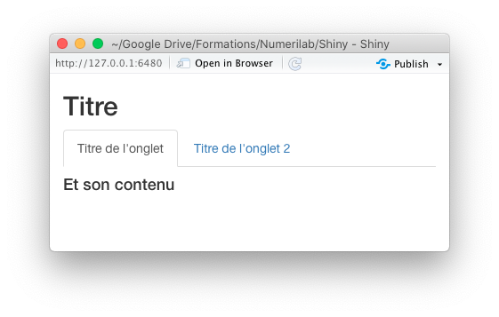
You can also organize your interface using tabs, with the tabsetPanel function, and defining each individual panel with the tabPanel function :
interface_onglets <- fluidPage(

  titlePanel("Titre"),

  tabsetPanel(
    tabPanel(
      "Titre de l'onglet",
      h4("Et son contenu")
    ),
    tabPanel(
      "Titre de l'onglet 2",
      h4("Et le contenu du deuxième onglet")
    )
  )

)
appli <- shinyApp(ui = interface_onglets, server = serveur_vide)
runApp(appli)
All these structures can also be combined. You could have for example a grid layout inside one of your tabs, and a panel layout inside another, etc.
There are many other options to organize the layout of your app, which are detailed here : https://shiny.rstudio.com/articles/layout-guide.html
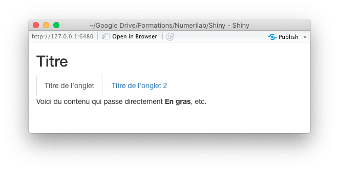
Finally, as the Shiny library’s work is to generate HTML code your web browser can interpret, you could also write your own HTML snippets to build your interface :
interface_html <- fluidPage(

  titlePanel("Titre"),

  tabsetPanel(
    tabPanel(
      "Titre de l'onglet",
      HTML("Voici du contenu qui passe directement <strong>En gras</strong>, etc.")
    ),
    tabPanel(
      "Titre de l'onglet 2",
      h4("Et le contenu du deuxième onglet")
    )
  )

)
appli <- shinyApp(ui = interface_html, server = serveur_vide)
runApp(appli)
So, if you or someone you know knows HTML, CSS or Javascript, the customization possibilities are endless!
Resources
In conclusion, here are some resources to guide your on your Shiny beginnings :
- RStudio’s cheat sheet, synthetizing on two pages the whole list of input and output controls available : https://shiny.rstudio.com/images/shiny-cheatsheet.pdf
- Written tutorials built by the Shiny team : https://shiny.rstudio.com/tutorial/#written-tutorials
- Video tutorials, also built by the Shiny team : https://shiny.rstudio.com/tutorial/#video-tutorials
- More in-depth articles about specific subjects (i.e. performance optimization, advanced customization, etc.) : https://shiny.rstudio.com/articles/