Functions and iteration
Charles Martin
February 2020
- Introduction
- When to write a function?
- Conditional execution
- Arguments
- Many exit points
- About the environment
- Introducing interation
- FOR loops
- The Map family of functions
- Managing issues
- There is also a map function to build data.frames
- data.frames on input *and * output
Introduction
Functions in R allow us to automate things, instead of copy-pasting code.
3 major advantages :
- Functions can have names, so it makes code easier to read
- If your requirements change, you only have one place where to change your code
- It minimises the risks associated with copy-pasting (e.g. forgetting to change a variable name, etc.)
When to write a function?
It is commonly recommended that start writing a function whenever you copy-paste some code for the second time (i.e. you have 3 copies of the code)
For example, if you have the relative abundance of species in 3 communities :
com1 = c(0.5,0.3,0.2)
com2 = c(0.7,0.2,0.1)
com3 = c(0.9,0.1)
You could calculate Shannon diversity for the first community with :
-sum(com1*log(com1))
[1] 1.029653
And then for the second and third one with :
-sum(com2*log(com2))
[1] 0.8018186
-sum(com3*log(com3))
[1] 0.325083
At this point, we’ve copy-pasted our code twice, so it is time to turn it into a function…
A good first step when writing a function is to determine what the function
needs, what are its inputs. In this case, the function needs the
relative abundances of a community. Let’s call them p, like in the traditional
notation.
p <- com1
-sum(p*log(p))
[1] 1.029653
p <- com2
-sum(p*log(p))
[1] 0.8018186
Notice that I immediately test my code, to make sure that I’ve extracted everything that I neede to make the code work.
Then, you only need to wrap this code and tell R that you function needs
one argument, p
If you don’t mention anything, a function in R returns the result of the last command it executes
diversite_shannon <- function(p) {
  -sum(p*log(p))
}
diversite_shannon(com1)
[1] 1.029653
diversite_shannon(com2)
[1] 0.8018186
diversite_shannon(com3)
[1] 0.325083
Our code is now much more readable AND easier to maintain
(yes, we’re still copy-pasting some stuff…)
Conditional execution
You can insert conditional statements inside your functions (anywhere in fact), using the if keyword
The typical structure of an IF statement goes like this :
if (condition) {
  # gets run if condition is true
} else {
  # gets run if condition is false
}
salutations <- function(nom) {
  if (nom == "Charles") {
   print("Allo Charles")
  } else {
    print("Qui êtes vous?")
  }
}
salutations("Esteban")
[1] "Qui êtes vous?"
salutations("Charles")
[1] "Allo Charles"
Note that it is optional for your function to return a value
Arguments
Functions in R can have as many arguments as you wish
Usually, in R, the first arguments contain data, whereas the last ones contain details about how to do the calculations.
These arguments about calculation details can have default values, which the user only has to change if needed.
pile_face <- function(n,probabilite_pile = 0.5) {
  sample(
    c("pile","face"),
    size = n,
    prob = c(probabilite_pile,1 - probabilite_pile),
    replace = TRUE
  )
}
pile_face(25)
 [1] "face" "face" "pile" "face" "face" "pile" "pile" "pile" "pile" "face"
[11] "pile" "pile" "face" "pile" "pile" "pile" "face" "pile" "face" "face"
[21] "pile" "face" "pile" "pile" "pile"
pile_face(25, 0.9)
 [1] "pile" "pile" "pile" "pile" "pile" "pile" "pile" "pile" "pile" "pile"
[11] "pile" "pile" "pile" "pile" "pile" "pile" "face" "pile" "pile" "pile"
[21] "face" "pile" "pile" "pile" "pile"
Defensive programming
When you become comfortable with writing functions, there will rapidly come a point where you won’t remember how you coded everything inside every function you’ve written and the constaints associated.
For example, our function to calculate Shannon’s diversity expects to receive
relative frequencies. The calculation is not defined if the sum of the p values
is not 1.
However, our function let’s us do the calculation on absolute numbers
diversite_shannon(c(1,5,25,12))
[1] -118.338
To protect our future-self, we can add some checks, which will stop the calculations if some condition is not met.
diversite_shannon <- function(p) {
  stopifnot(sum(p) == 1)
  - sum(p*log(p))
}
diversite_shannon(c(1,5,25,12))
Error in diversite_shannon(c(1, 5, 25, 12)): sum(p) == 1 is not TRUE
You can also write more user-friendly messages with just a little more code
diversite_shannon <- function(p) {
  if (sum(p) != 1) {
    stop("L'argument p doit contenir des probabilités relatives, dont la somme est 1.")
  }
  - sum(p*log(p))
}
diversite_shannon(c(1,5,25,12))
Error in diversite_shannon(c(1, 5, 25, 12)): L'argument p doit contenir des probabilités relatives, dont la somme est 1.
The special dot-dot-dot (…) argument
Function definitions in R can also contain a special argument named dot-dot-dot. This argument, if present, will catch every argument that the function received and was not explicitely named in the function definition.
It can be especially useful to send these arguments back to another function.
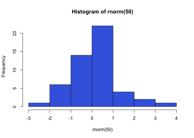
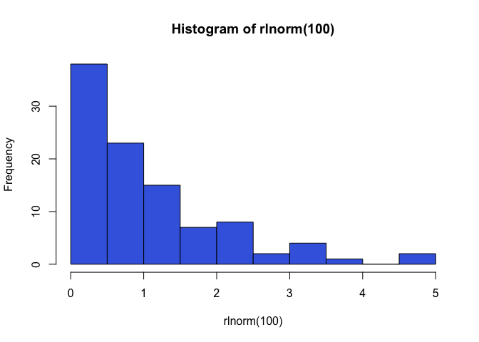
If anytime you need an histogram you like to have it blue instead of white, you could create your own function, which calls the original, adding you favorite or often used options:
bleustogram <- function(...){
  hist(..., col = "royalblue")
}
bleustogram(rnorm(50))

bleustogram(rlnorm(100))

Many exit points
An R function can contain many points where it stops to return a value. In this case, these points need to be defined explicitely :
diversite <- function(p, indice = "shannon") {
  if (indice == "shannon") {
    return(-sum(p*log(p)))
  } else if (indice == "simpson") {
    return(sum(p^2))
  } else {
    stop("L'indice doit être shannon ou simpson")
  }
}
diversite(c(0.5,0.3,0.2))
[1] 1.029653
diversite(c(0.5,0.3,0.2), indice = "simpson")
[1] 0.38
About the environment
Anything that you create inside a function exist only there, and cannot be accessed from the outside. Objects are reset every the functio is called.
A special feature of R is that, if a variable is not defined inside a function, R will also search outside of it, in the global environment, for an object having the same name.
b <- 2
f1 <- function(d) {
  d * b
}
f1(3)
[1] 6
f2 <- function(d) {
  b <- 8
  d * b
}
f2(3)
[1] 24
b
[1] 2
d
Error in eval(expr, envir, enclos): object 'd' not found
This is why it is important to be very careful while extracting the arguments necessary to your function. It is important to restart your R session once in a while, to make sure that things are not “accidently working” because an object with a particular name exist in your working environment.
Introducing interation
Beside function, another programming technique to reduce code duplication is the use of iterations (syn. repetitions)
There are two styles of iteration in R : Imperative programming and functional programming.
Imperative programming includes FOR and WHILE loops. It is often the most intuitive way to begin, because the concepts are explicit.
Consequently, imperative programming involves lots of “plumbing code”, that repeats itself from a loop to another and “drowns” the actual intent of the code. Functional programming allows us to extract to the core task of our code and produces denser, easier to read and maintain code.
FOR loops
Let’s start with the Baby Shark lyrics : https://genius.com/Pinkfong-baby-shark-lyrics
If one wanted to automate the writing of the first verse of the song, we could write :
for (i in 1:3) {
  print("Baby shark, doo doo doo doo doo doo")
}
print("Baby shark!")
[1] "Baby shark, doo doo doo doo doo doo"
[1] "Baby shark, doo doo doo doo doo doo"
[1] "Baby shark, doo doo doo doo doo doo"
[1] "Baby shark!"
A FOR loop has 2 main components :
- The first line defines how many times we wish to do the loop
- The code between {} defines the code we wish to repeat.
Each iteration doesn’t need to do an identical job, their action can be customized based on the index the loop is currently at.
mots = c("Baby shark","Mommy shark","It's the end")
for (i in seq_along(mots)) { # vs. 1:length(mots)
  print(paste0(mots[i],", doo doo doo doo doo doo"))
}
[1] "Baby shark, doo doo doo doo doo doo"
[1] "Mommy shark, doo doo doo doo doo doo"
[1] "It's the end, doo doo doo doo doo doo"
Nesting
You probably saw that one coming from a mile, but you can also nest loops inside one another:
mots = c("Baby shark","Mommy shark","It's the end")
for (i in seq_along(mots)) {
  for (j in 1:3) {
    print(paste0(mots[i],", doo doo doo doo doo doo"))
  }
  print(paste0(mots[i],"!"))
}
[1] "Baby shark, doo doo doo doo doo doo"
[1] "Baby shark, doo doo doo doo doo doo"
[1] "Baby shark, doo doo doo doo doo doo"
[1] "Baby shark!"
[1] "Mommy shark, doo doo doo doo doo doo"
[1] "Mommy shark, doo doo doo doo doo doo"
[1] "Mommy shark, doo doo doo doo doo doo"
[1] "Mommy shark!"
[1] "It's the end, doo doo doo doo doo doo"
[1] "It's the end, doo doo doo doo doo doo"
[1] "It's the end, doo doo doo doo doo doo"
[1] "It's the end!"
Keeping a result for each iteration
In a loop, it is often useful to keep the result of some calculation at each iteration. In such a case, it is strongly recommended to pre-allocate our result object before the loop begins. This is the key to fast loops in R.
For example, let’s prepare a loop that would calculate the absolute value of a series of numbers
nombres <- c(-1,0,1,-5)
valeurs_absolues <- vector("double", length(nombres))
for (i in seq_along(nombres)) {
  valeurs_absolues[i] <- abs(nombres[i])
}
valeurs_absolues
[1] 1 0 1 5
Unknown number of iterations
When you don’t know beforehand how many times our loop will run, there
exist a second R structure which allows this kind of iteration :
the while loop.
These loops are particularly useful in simulations.
For example, let’s run some code to determine how many coin tosses are needed to obtain a sequence of 3 heads in a row.
tirages <- 0
piles_de_suite <- 0

while (piles_de_suite < 3) {

  resultat <- pile_face(1)

  if ((resultat) == "pile") {
    piles_de_suite <- piles_de_suite + 1
  } else {
    piles_de_suite <- 0
  }

  tirages <- tirages + 1
}

tirages
[1] 33
The Map family of functions
As said before, iteration can be tackly in a completely different way, using functionnal programming. In R, the purrr package contains many functions that allows us to do functional programming in a simple and intuitive way.
library(purrr)
The principle behind each of these functions is all the same : instead of writing the code that makes the loop work, you give it a function and a series of elements to apply it on.
There are many map functions, depending on the return type you want
to obtain.
mapreturns a listmap_lglreturnsTRUE/FALSEmap_intreturns integersmap_dblreturns floating point numbersmap_chrreturns textmap_dfreturns a data.frame object
Let’s revisit our code snippet about absolute values. It could be converted to this simple piece of code
nombres <- c(-1,0,1,-5)
valeurs_absolues <- map_dbl(nombres, abs)
valeurs_absolues
[1] 1 0 1 5
We thus save a lot of plumbing code about how to make that loop
You can also give map a custom made function, e.g. let’s say you wanted
to calculate the absolute value of these numbers and then add 10.
nombres <- c(-1,0,1,-5)
ma_fonction <- function(x) {
  abs(x) + 10
}
map_dbl(nombres, ma_fonction)
[1] 11 10 11 15
If this custom made function is used only in this code, you can define it anonymously inside the map function :
nombres <- c(-1,0,1,-5)
map_dbl(nombres, function(x) {abs(x) + 10})
[1] 11 10 11 15
Generally, this use is limited to short pieces of code.
Les raccourcis inclus
Shortcuts included in map functions
One of the advantages of the map functions in purrr package is that
it enables us to cut the obvious parts of our code with shortcuts :
  nombres <- c(-1,0,1,-5)
  map_dbl(nombres, ~ abs(.) + 10)
[1] 11 10 11 15
You can replace the function part with a ~ and the name of the
variable with a dot.
Managing issues
When using map functions on long series of data, it can happen that our
function fails for a reason or another.
When a problem happens, the map function stops, with an error message, but
you don’t retrieve all the instances that worked before the issue.
Let’s go back to our Shannon diversity function. If one of our communities does not contain relative frequencies, we loose all the remaining results…
communautes <- list(
  c(0.5,0.3,0.2),
  c(0.9,0.1),
  c(10,3,1)
)

map_dbl(communautes,diversite_shannon)
Error in .f(.x[[i]], ...): L'argument p doit contenir des probabilités relatives, dont la somme est 1.
The purrr package contains many adverbs to manage these kinds of situations.
In each case, these adverbs wrap our function by modifying it’s behaviour in
case of errors. Here we’re only seing the simplest case, possibly, to which you need to supply a value in case of error.
map_dbl(communautes,possibly(diversite_shannon,NA))
[1] 1.029653 0.325083 NA
There is also a map function to build data.frames
map_df(communautes,function(x){
  data.frame(
    richesse = length(x),
    shannon = diversite(x, indice = "shannon"),
    simpson = diversite(x, indice = "simpson")
  )
})
  richesse    shannon simpson
1        3   1.029653    0.38
2        2   0.325083    0.82
3        3 -26.321688  110.00
This function can also me tremendously useful when you need to read a bunch of csv files from a folder and bind them in a single data.frame
fichiers <- list.files(
  "/Dossier/Avec/Les/Donnees",
  pattern = "*.csv",
  full.names = TRUE
)
tableau <- map_df(fichiers,read.csv)
data.frames on input *and * output
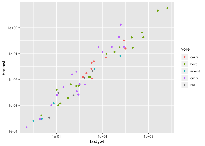
To illustrate this case, let’s imagine a scenario where you have explored the relationship between body weight and brain weight in mammals.
library(ggplot2)
library(dplyr)
Attaching package: 'dplyr'
The following objects are masked from 'package:stats':

    filter, lag
The following objects are masked from 'package:base':

    intersect, setdiff, setequal, union
data(msleep)

msleep %>%
  ggplot(aes(x = bodywt, y = brainwt)) +
  geom_point(aes(color = vore)) +
  scale_x_log10() +
  scale_y_log10()
Warning: Removed 27 rows containing missing values (geom_point).

You would now like to run a regression per group to compare the parameter values.
First, let’s see how we’d do that for a single group, the herbivores :
x <- msleep %>% filter(vore == "herbi")
m <- lm(log(brainwt)~log(bodywt),data = x)
summary(m)
Call:
lm(formula = log(brainwt) ~ log(bodywt), data = x)

Residuals:
     Min       1Q   Median       3Q      Max
-0.79504 -0.28970 -0.08648  0.19723  1.12209

Coefficients:
            Estimate Std. Error t value Pr(>|t|)
(Intercept) -4.94213    0.12464  -39.65  < 2e-16 ***
log(bodywt)  0.74212    0.03007   24.68 2.48e-15 ***
---
Signif. codes:  0 '***' 0.001 '**' 0.01 '*' 0.05 '.' 0.1 ' ' 1

Residual standard error: 0.4864 on 18 degrees of freedom
  (12 observations deleted due to missingness)
Multiple R-squared:  0.9713,	Adjusted R-squared:  0.9697
F-statistic: 609.1 on 1 and 18 DF,  p-value: 2.484e-15
It is not necessarily simple to extract the slope estimate from this model object to put them in a data.frame object.
str(m)
List of 13
 $ coefficients : Named num [1:2] -4.942 0.742
  ..- attr(*, "names")= chr [1:2] "(Intercept)" "log(bodywt)"
 $ residuals    : Named num [1:20] -0.6656 0.6216 0.1733 -0.0253 0.5345 ...
  ..- attr(*, "names")= chr [1:20] "2" "4" "5" "6" ...
 $ effects      : Named num [1:20] 15.3808 12.0043 0.3263 -0.0469 0.4878 ...
  ..- attr(*, "names")= chr [1:20] "(Intercept)" "log(bodywt)" "" "" ...
 $ rank         : int 2
 $ fitted.values: Named num [1:20] -0.195 -2.942 -2.336 -5.178 -5.586 ...
  ..- attr(*, "names")= chr [1:20] "2" "4" "5" "6" ...
 $ assign       : int [1:2] 0 1
 $ qr           :List of 5
  ..$ qr   : num [1:20, 1:2] -4.472 0.224 0.224 0.224 0.224 ...
  .. ..- attr(*, "dimnames")=List of 2
  .. .. ..$ : chr [1:20] "2" "4" "5" "6" ...
  .. .. ..$ : chr [1:2] "(Intercept)" "log(bodywt)"
  .. ..- attr(*, "assign")= int [1:2] 0 1
  ..$ qraux: num [1:2] 1.22 1.01
  ..$ pivot: int [1:2] 1 2
  ..$ tol  : num 1e-07
  ..$ rank : int 2
  ..- attr(*, "class")= chr "qr"
 $ df.residual  : int 18
 $ na.action    : 'omit' Named int [1:12] 1 3 12 13 15 17 19 21 22 25 ...
  ..- attr(*, "names")= chr [1:12] "1" "3" "12" "13" ...
 $ xlevels      : Named list()
 $ call         : language lm(formula = log(brainwt) ~ log(bodywt), data = x)
 $ terms        :Classes 'terms', 'formula'  language log(brainwt) ~ log(bodywt)
  .. ..- attr(*, "variables")= language list(log(brainwt), log(bodywt))
  .. ..- attr(*, "factors")= int [1:2, 1] 0 1
  .. .. ..- attr(*, "dimnames")=List of 2
  .. .. .. ..$ : chr [1:2] "log(brainwt)" "log(bodywt)"
  .. .. .. ..$ : chr "log(bodywt)"
  .. ..- attr(*, "term.labels")= chr "log(bodywt)"
  .. ..- attr(*, "order")= int 1
  .. ..- attr(*, "intercept")= int 1
  .. ..- attr(*, "response")= int 1
  .. ..- attr(*, ".Environment")=<environment: R_GlobalEnv>
  .. ..- attr(*, "predvars")= language list(log(brainwt), log(bodywt))
  .. ..- attr(*, "dataClasses")= Named chr [1:2] "numeric" "numeric"
  .. .. ..- attr(*, "names")= chr [1:2] "log(brainwt)" "log(bodywt)"
 $ model        :'data.frame':	20 obs. of  2 variables:
  ..$ log(brainwt): num [1:20] -0.86 -2.32 -2.16 -5.2 -5.05 ...
  ..$ log(bodywt) : num [1:20] 6.397 2.695 3.512 -0.317 -0.868 ...
  ..- attr(*, "terms")=Classes 'terms', 'formula'  language log(brainwt) ~ log(bodywt)
  .. .. ..- attr(*, "variables")= language list(log(brainwt), log(bodywt))
  .. .. ..- attr(*, "factors")= int [1:2, 1] 0 1
  .. .. .. ..- attr(*, "dimnames")=List of 2
  .. .. .. .. ..$ : chr [1:2] "log(brainwt)" "log(bodywt)"
  .. .. .. .. ..$ : chr "log(bodywt)"
  .. .. ..- attr(*, "term.labels")= chr "log(bodywt)"
  .. .. ..- attr(*, "order")= int 1
  .. .. ..- attr(*, "intercept")= int 1
  .. .. ..- attr(*, "response")= int 1
  .. .. ..- attr(*, ".Environment")=<environment: R_GlobalEnv>
  .. .. ..- attr(*, "predvars")= language list(log(brainwt), log(bodywt))
  .. .. ..- attr(*, "dataClasses")= Named chr [1:2] "numeric" "numeric"
  .. .. .. ..- attr(*, "names")= chr [1:2] "log(brainwt)" "log(bodywt)"
  ..- attr(*, "na.action")= 'omit' Named int [1:12] 1 3 12 13 15 17 19 21 22 25 ...
  .. ..- attr(*, "names")= chr [1:12] "1" "3" "12" "13" ...
 - attr(*, "class")= chr "lm"
m$coefficients
(Intercept) log(bodywt)
  -4.942134    0.742122
In the tidyverse, there is a package made especially for such situations, to extract numbers from models and put them in a data.frame.
library(broom)
tidy(m)
# A tibble: 2 x 5
  term        estimate std.error statistic  p.value
  <chr>          <dbl>     <dbl>     <dbl>    <dbl>
1 (Intercept)   -4.94     0.125      -39.6 5.69e-19
2 log(bodywt)    0.742    0.0301      24.7 2.48e-15
You could also have been interest in model-level numbers instead :
glance(m)
# A tibble: 1 x 11
  r.squared adj.r.squared sigma statistic  p.value    df logLik   AIC   BIC
      <dbl>         <dbl> <dbl>     <dbl>    <dbl> <int>  <dbl> <dbl> <dbl>
1     0.971         0.970 0.486      609. 2.48e-15     2  -12.9  31.8  34.8
# … with 2 more variables: deviance <dbl>, df.residual <int>
Now we have in hand everything we need to calculate a regression model per group
resultats <- msleep %>%
  group_by(vore) %>%
  group_modify(function(x,...){
    m <- lm(log(brainwt)~log(bodywt),data = x)
    tidy(m)
  })
resultats
# A tibble: 10 x 6
# Groups:   vore [5]
   vore    term        estimate std.error statistic  p.value
   <chr>   <chr>          <dbl>     <dbl>     <dbl>    <dbl>
 1 carni   (Intercept)   -4.47     0.278     -16.1  8.61e- 7
 2 carni   log(bodywt)    0.667    0.112       5.95 5.71e- 4
 3 herbi   (Intercept)   -4.94     0.125     -39.6  5.69e-19
 4 herbi   log(bodywt)    0.742    0.0301     24.7  2.48e-15
 5 insecti (Intercept)   -5.11     0.167     -30.6  7.66e- 5
 6 insecti log(bodywt)    0.702    0.0477     14.7  6.84e- 4
 7 omni    (Intercept)   -4.45     0.202     -22.0  7.76e-13
 8 omni    log(bodywt)    0.869    0.0724     12.0  4.28e- 9
 9 <NA>    (Intercept)   -4.97     0.345     -14.4  7.23e- 4
10 <NA>    log(bodywt)    0.837    0.194       4.33 2.28e- 2
See that, just as when building functions, we made sure to test our code before integrating in the iteration code
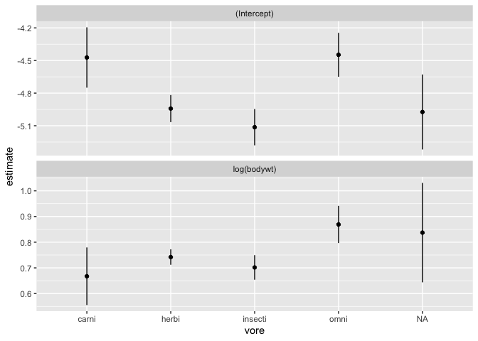
You can then vizualize all these coefficients in a single, synthetic plot.
resultats %>%
  ggplot(aes(x = vore, y = estimate)) +
  geom_point() +
  geom_linerange(aes(ymin = estimate-std.error, ymax = estimate+std.error)) +
  facet_wrap(~term, scale = "free_y", ncol = 1)
