Example of pseudo-replication & ANOVA and post-hoc analysis
Fan Qin & Roxanne Giguère-Tremblay
May 2021
- Section 1 : Examples of replication and pseudo-replication
- Section 2: Analysis of variance and post-hoc analysis
- Section 3: Exercises
- 1. Compute one-way anova with an independent factor (example of category)
- 2. Verify the normality of the data, and choose the right data transformation
- 3. Pairwaise comparison with emmeans package
- 4. Compute a two-way anova
- 5. Checking assumptions
- 6. Models selection
- 7. Interpreting output of analysis of variance
- 8. Pairwise comparison
The script was designed by Fan Qin (workshop facilitator) and revised by Roxanne Giguère-Tremblay (Co-facilitator). This workshop was presented at the Joint Symposium on Ecotoxicology (May 2021).
# Packages
# Here are the packages that will be used to define the basic functions.
library(dplyr) # alternative installation for the function of '%>%'
# package for data visualization
library(ggplot2)
library(ggpubr)
# package for post-hoc comparison
library(emmeans)
# package allowing you to make Type-I, Type-II or Type-III ANOVA
library(car)
Section 1 : Examples of replication and pseudo-replication
Context:
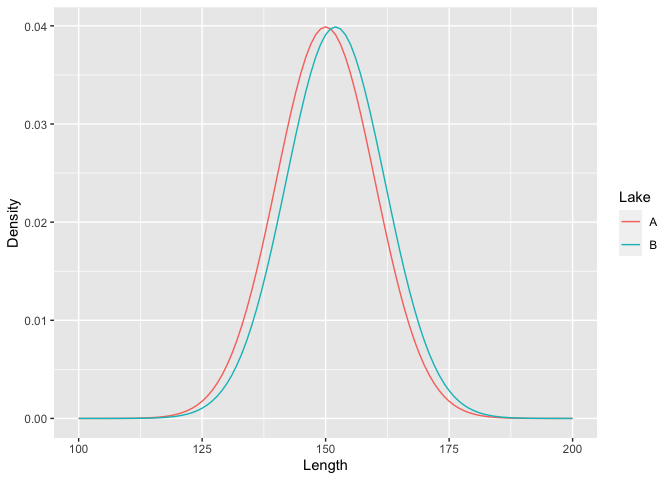
We want to compare the length of the same fish species between two lakes A and B. The length distribution is assumed to follow a normal distribution.
* Lake A population: mean = 150 and sd = 10
* Lake B population: mean = 152 and sd = 10

The mean length of the fish population in lake B is two units higher than the mean length of the fish population in lake A (i.e., 152 in lake B vs. 150 in lake A). For simplicity, we choose here homogeneous populations (same standard deviation, *sd*). It is possible to visualize the theoretical distribution of these two populations.
muA = 150
sigmaA = 10

muB = 152
sigmaB = 10

x = seq(100,200,1)

dA = dnorm(x,mean=muA,sd=sigmaA)
dB = dnorm(x,mean=muB,sd=sigmaB)

Density = c(dA,dB)
Length = c(x,x)
Lake = c(rep("A",length(x)),rep("B",length(x)))
Data = data.frame(Length,Density,Lake)

# We use the ggplot2 package to view data on a chart
ggplot(data=Data, aes(Length,Density,col=Lake))+
  geom_line()
1. Replication
From this context, suppose we want to compare fish lengths between these two lakes:
Scenario 1
1 individual is sampled per lake.
n=1
sampleA = rnorm(n,mean=muA,sd=sigmaA)
sampleB = rnorm(n,mean=muB,sd=sigmaB)
Let’s compare these two samples using a Student’s t-test.
t.test(sampleA,sampleB,var.equal=TRUE)
Warning message:
Error in t.test.default(sampleA, sampleB, var.equal = TRUE) :
  not enough observations Conclusion: we need replication to perform statistical analysis
Scenario 2
10 individuals are sampled per lake.
n=10
sampleA = rnorm(n,mean=muA,sd=sigmaA)
sampleB = rnorm(n,mean=muB,sd=sigmaB)
Let’s compare these two samples using a Student’s t-test.
t.test(sampleA,sampleB,var.equal=TRUE)
##
## 	Two Sample t-test
##
## data:  sampleA and sampleB
## t = -0.3627, df = 18, p-value = 0.7211
## alternative hypothesis: true difference in means is not equal to 0
## 95 percent confidence interval:
##  -11.440849   8.072177
## sample estimates:
## mean of x mean of y
##  149.2165  150.9008
Conclusion: Student’s t-test compares the mean of the two samples, but no significant difference was detected with 10 replicates (P>0.05).
Scenario 3
1000 individuals are sampled per lake.
n=1000
sampleA = rnorm(n,mean=muA,sd=sigmaA)
sampleB = rnorm(n,mean=muB,sd=sigmaB)
Let’s compare these two samples using a Student’s t-test.
t.test(sampleA,sampleB,var.equal=TRUE)
##
## 	Two Sample t-test
##
## data:  sampleA and sampleB
## t = -4.7875, df = 1998, p-value = 1.813e-06
## alternative hypothesis: true difference in means is not equal to 0
## 95 percent confidence interval:
##  -3.023632 -1.266294
## sample estimates:
## mean of x mean of y
##  150.0463  152.1912
Conclusion: by increasing the number of replicates, the test is now significant (P<0.001)
It is important to note that in all three scenarios the populations have not changed! We should therefore have similar biological interpretations. Increasing the number of replicates makes it possible to detect increasingly small differences.
2. Pseudo-replication
Let’s take the example of scenario 2. Suppose this time that each individual is measured 3 times, without measurement error. This is artificially equivalent to a threefold increase in the sample size, which is a mistake.
Here is a demonstration:
Scenario with pseudo-replication.
We sampled ten individuals per lake, each individual is measured three times.
n=10

sampleA = rnorm(n,mean=muA,sd=sigmaA)
sampleB = rnorm(n,mean=muB,sd=sigmaB)

t.test(sampleA,sampleB,var.equal=TRUE) #t-test before pseudo-replication
##
## 	Two Sample t-test
##
## data:  sampleA and sampleB
## t = -0.53133, df = 18, p-value = 0.6017
## alternative hypothesis: true difference in means is not equal to 0
## 95 percent confidence interval:
##  -14.092969   8.403512
## sample estimates:
## mean of x mean of y
##  148.2262  151.0710
sampleA = c(sampleA,sampleA,sampleA) #Repeat sample A three times
sampleB = c(sampleB,sampleB,sampleB) #Repeat sample A three times

t.test(sampleA,sampleB,var.equal=TRUE) #t-test after pseudo-replication
##
## 	Two Sample t-test
##
## data:  sampleA and sampleB
## t = -0.95377, df = 58, p-value = 0.3442
## alternative hypothesis: true difference in means is not equal to 0
## 95 percent confidence interval:
##  -8.815077  3.125620
## sample estimates:
## mean of x mean of y
##  148.2262  151.0710
Conclusion: By comparing the two Student’s t-test (before and after the pseudo-replication, you can see how much the p-value is reduced after the pseudo-replication (and some times wrongly significant) whereas the mean estimates are the same. Mixed modelling is a good alternative to deal with repeated measures, but this is beyond the scope of this workshop
Section 2: Analysis of variance and post-hoc analysis
1. Arranging data
In the database that will be used, the data arrangement goes as follows:
             variable1      variable2    variable3
sample1
sample2
sample3
2. Reading data
Context:
Study the effects of multiple factors on the concentration of MeHg in three laks (with 45 observations and 5 variables)
# For Windows users - use '/' not '\' in the script for the direction of file
# setwd('C:/Users/sabic/OneDrive/Documents/UQTR/DONN? ES-field-lab/seminar2')
# getwd()

# If you are in a R projet and the data file is at the root of this project, you can simply run
workshop<-read.csv("Mercure2002_1.csv")

# Or if your data is in the .txt format, use the function read.delim as follow
# workshop <- read.delim("Mercure2002.txt")
# View the data table
View(workshop)
# Get the structural information of the data
str(workshop)
# Change data properties
# Numeric to character example
workshop$station<-as.character(workshop$station)

# In the case if the independent variable name is incorrectly recognized by R, you can use the
# next way to change the name.
names(workshop)[1]<-"lake"
# Or
# names(workshop)[names(workshop)=="i...lac"]<- 'lake'
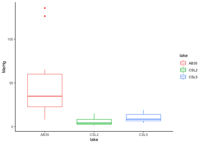
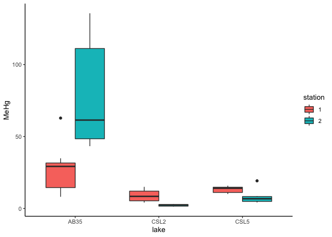
3. Data visualization
Boxplot is the best way to visualize quantitative data according to a qualitative variable
ggplot(data=workshop, aes(x=lake, y=MeHg,color=lake))+
  geom_boxplot(width=0.7,na.rm = TRUE)+
  theme_classic()
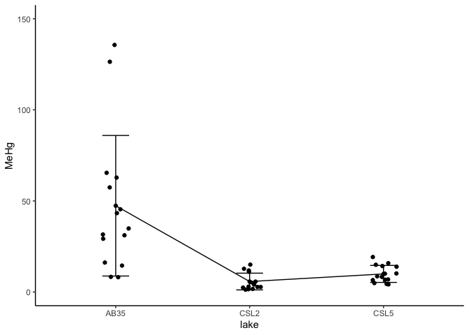
Or if you want to visualize data points with mean and standard deviation
# Step 1 : calculate mean and sd
workshop_stat   = aggregate(MeHg~lake,data=workshop, mean)
workshop_sd     = aggregate(MeHg~lake,data=workshop,sd)
workshop_stat$sd=workshop_sd[,2]
# Step 2 : ggplot2
ggplot(workshop_stat, aes(x=lake, y=MeHg,group = 1)) +
  geom_point(color="black",na.rm = T) +
  geom_errorbar(aes(ymin=MeHg-sd, ymax=MeHg+sd),width = 0.2)+ylim(0,150)+
  geom_point(data=workshop, position = position_jitter(w = 0.1, h = 0))+ # add points
  geom_path(aes(y=MeHg))+theme_classic()
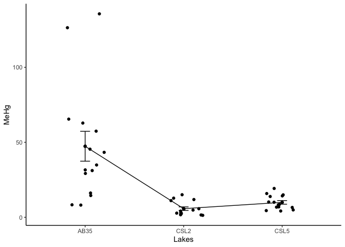
Or use the ggpubr package for rapid visualization.
ggline(workshop, x = "lake", y = "MeHg",
       add = c("mean_se", "jitter"),
       order = c("AB35", "CSL2","CSL5"), # Optionnal: you can change the order of the categories
       ylab = "MeHg", xlab = "Lakes")+theme_classic()
4. Compute one-way ANOVA
There are two ways of doing ANOVA that will be presented in this workshop
Way 1 with the aov() function
res.aov <- aov(MeHg ~ lake, data = workshop)
summary(res.aov)
##             Df Sum Sq Mean Sq F value  Pr(>F)
## lake         2  15741    7870   15.42 9.5e-06 ***
## Residuals   42  21432     510
## ---
## Signif. codes:  0 '***' 0.001 '**' 0.01 '*' 0.05 '.' 0.1 ' ' 1
In the summary, we can see a significant difference between lakes on the concentration of MeHg, but we cannot distinguish which lake contributes to the significance.
Way 2 with the lm() function
mod<-lm(formula= (MeHg) ~ lake, data = workshop)
summary(mod)
##
## Call:
## lm(formula = (MeHg) ~ lake, data = workshop)
##
## Residuals:
##     Min      1Q  Median      3Q     Max
## -39.232  -4.449  -1.938   5.016  88.265
##
## Coefficients:
##             Estimate Std. Error t value Pr(>|t|)
## (Intercept)   47.366      5.833   8.121 3.80e-10 ***
## lakeCSL2     -41.600      8.249  -5.043 9.25e-06 ***
## lakeCSL5     -37.419      8.249  -4.536 4.72e-05 ***
## ---
## Signif. codes:  0 '***' 0.001 '**' 0.01 '*' 0.05 '.' 0.1 ' ' 1
##
## Residual standard error: 22.59 on 42 degrees of freedom
## Multiple R-squared:  0.4235,	Adjusted R-squared:  0.396
## F-statistic: 15.42 on 2 and 42 DF,  p-value: 9.496e-06
lm() can make pairwise-comparison under a limited condition, here it seems that the concentration of MeHg in lake AB35 is significantly different than lake CSL2 and CSL5.
The concentration of MeHg in Lake AB35 was used as the baseline to make the comparison.
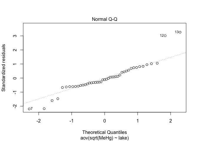
5. Checking assumptions
The two main assumptions to check are the normality of residuals and homogneity of variances There are several tests to check normality, e.g. Shapiro-Wilk test, Levene’s test Here we recommend an easier and visual way by plotting normality with aov() or lm()
# with aov()
plot(res.aov,1) # Look at the homogeneity of variances
plot(res.aov,2) # Look at the normality of residuals
# with lm()
plot(mod,1) # Look at the homogeneity of variances
plot(mod,2) # Look at the normality of residuals
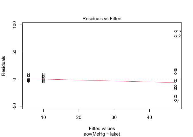

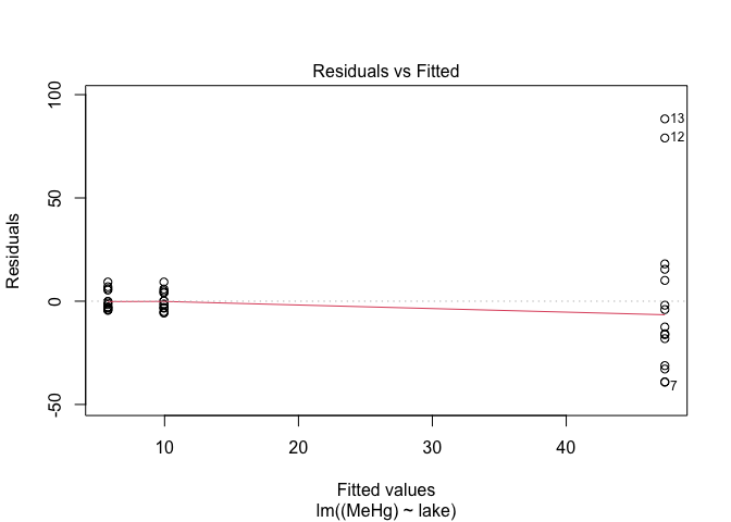
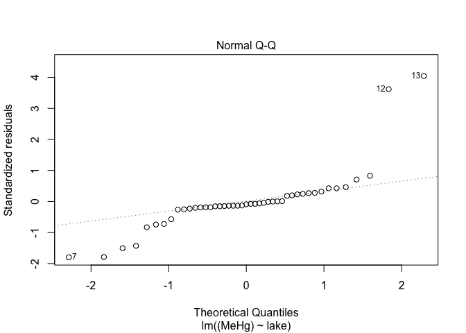
The spread of points on the first graph increase according to fitted values, indicating variance heterogeneity. The points on the second graph deviate from the line, indicating that the residuals are not normally distributed.
6. Transform data to satisfy normality
Log transform your data to achieve normality. Other functions are available (like the root-square function) but the log function is commonly used and should be your first attempt
res.aov1 <- aov(log(MeHg) ~ lake, data = workshop)  # log transform
res.aov2 <- aov(sqrt(MeHg) ~ lake, data = workshop) # root-square transform
plot(res.aov,2)
plot(res.aov1,2)
plot(res.aov2,2)

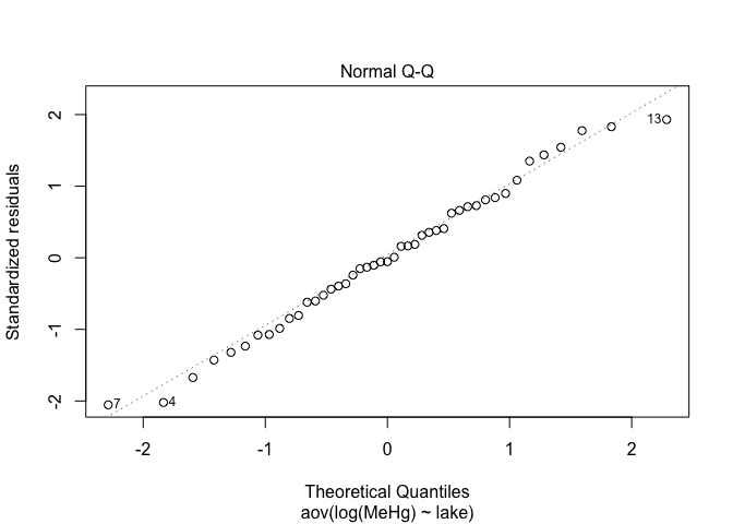
Alignment of points along the line is better when data are log-transformed. This is definitively the best option in this case
7. Pairwais-comparison for one-way ANOVA
When applying post hoc pairwais comparison, it is important to correct the p-value when performing multiple analysis of variance on the same database, to avoid type I error, including accepting a false H1 (False Positive)
Way 1: Tukey HSD (Tukey Honest Significant Differences)
TukeyHSD(res.aov1)
##   Tukey multiple comparisons of means
##     95% family-wise confidence level
##
## Fit: aov(formula = log(MeHg) ~ lake, data = workshop)
##
## $lake
##                 diff         lwr        upr     p adj
## CSL2-AB35 -2.0902346 -2.73890503 -1.4415641 0.0000000
## CSL5-AB35 -1.3555587 -2.00422912 -0.7068882 0.0000244
## CSL5-CSL2  0.7346759  0.08600546  1.3833464 0.0232184
The p-values have been adjusted in the output of this function with Tukey’s ‘Honest Significant Difference’ method
Way 2: Emmeans package with customized p-value adjustment
emmeans() function in Emmeans package allows to customize the correction methods
# p-value adjustment types: holm, tukey, none, sidak, etc.
res.emm <- emmeans(res.aov1,  pairwise ~ lake, adjust ="tukey")
res.emm$contrasts %>% summary(infer = TRUE) %>% as.data.frame()
##      contrast   estimate        SE df   lower.CL    upper.CL   t.ratio
## 1 AB35 - CSL2  2.0902346 0.2669982 42  1.4415641  2.73890503  7.828647
## 2 AB35 - CSL5  1.3555587 0.2669982 42  0.7068882  2.00422912  5.077033
## 3 CSL2 - CSL5 -0.7346759 0.2669982 42 -1.3833464 -0.08600546 -2.751614
##        p.value
## 1 2.903029e-09
## 2 2.435678e-05
## 3 2.321839e-02
res.emm.2 <- emmeans(res.aov1,  pairwise ~ lake, adjust ="holm")
res.emm.2$contrasts %>% summary(infer = TRUE) %>% as.data.frame()
##      contrast   estimate        SE df  lower.CL    upper.CL   t.ratio
## 1 AB35 - CSL2  2.0902346 0.2669982 42  1.424430  2.75603928  7.828647
## 2 AB35 - CSL5  1.3555587 0.2669982 42  0.689754  2.02136337  5.077033
## 3 CSL2 - CSL5 -0.7346759 0.2669982 42 -1.400481 -0.06887122 -2.751614
##        p.value
## 1 2.916571e-09
## 2 1.657414e-05
## 3 8.716465e-03
Significant differences are observed in all pairwise comparisons in this case.
Other packages and functions: e.g. the glht() function in the multcomp package.
8. Two-way ANOVA
Two-way ANOVA implies a quantitative response variable and two factors. We will take the same exemple as above but adding the station as a new factor
# Use the same dataset
# Set explicative variables as categoric variables
workshop$station<-as.factor(workshop$station)
workshop$lake<-as.factor(workshop$lake)
# View and verify structural information for the dataset
str(workshop)
## 'data.frame':	45 obs. of  5 variables:
##  $ lake               : Factor w/ 3 levels "AB35","CSL2",..: 1 1 1 1 1 1 1 1 1 1 ...
##  $ station            : Factor w/ 2 levels "1","2": 1 1 1 1 1 1 1 1 1 2 ...
##  $ replicat           : int  1 1 1 2 2 2 3 3 3 1 ...
##  $ replicat_analytique: int  1 2 3 1 2 3 1 2 3 1 ...
##  $ MeHg               : num  62.82 31.61 34.89 8.33 31.15 ...
# Data visualization
ggplot(data=workshop, aes(x=lake, y=MeHg,fill=station))+
geom_boxplot(width=0.7,na.rm = TRUE,position = position_dodge(0.7))+
theme_classic()
# Or
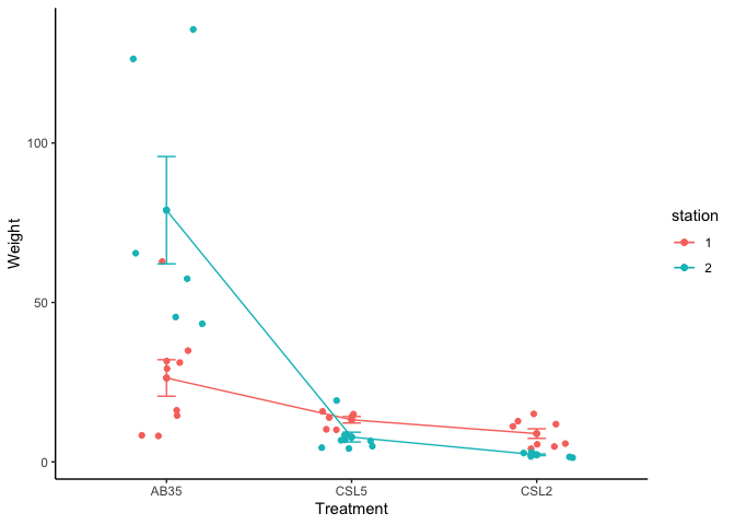
ggline(workshop, x = "lake", y = "MeHg", group='station', color = 'station',
add = c("mean_se", "jitter"),
order = c("AB35", "CSL5", "CSL2"),
ylab = "Weight", xlab = "Treatment")+theme_classic()
8.1 Different types of multipe-way ANOVA (including two-way ANOVA)
In R, default setting is always type I or type II with the foncitons anova(), or aov(). The “car” package can help specify the type of ANOVA with the Anova() function. Type III makes more sense for studies in ecology or ecotoxicology. The lm() function uses type III automatically.
The different types could briefly describe as following:
Type I  : assign the variation to different variables in a sequential order

Type II : No interaction between explicive variables, the variation is attributed to one explisive variable takes into account of others.

Type III: With interactions between explicive variables, same way to assign variation as Type II.
It is comparably easy to find detail description of the 3 type of ANOVA on internet
8.2 Model Selection - Establish Model - Linear Model
When we have > = 2 independent factors, we can establish linear models according to the relationships between the independent variables. We will use Aikaike Information Criterion (AIC) to compare and select the best model.
mod1<-lm(formula = log(MeHg) ~ lake, data=workshop) # Effect of the lake
mod2<-lm(formula = log(MeHg) ~ station, data=workshop) # Effect of the sampling station
mod3<-lm(formula = log(MeHg) ~ lake + station, data=workshop) # Additive effect of the lake and the station
mod4<-lm(formula = log(MeHg) ~ lake + station + lake*station, data=workshop) # with interaction
# Uses AIC to select the right model for subsequent scans
# the best model has the smallest value of AIC
AIC(mod1,mod2,mod3,mod4)
##      df       AIC
## mod1  4 104.42422
## mod2  3 142.26533
## mod3  5 104.87350
## mod4  7  71.50172
#You can order models with the ‘model.sel’ function of the MuMIn package
library(MuMIn)
model.sel(mod1,mod2,mod3,mod4)
## Model selection table
##      (Int) lak stt lak:stt             family df  logLik  AICc delta weight
## mod4 3.071   +   +       + gaussian(identity)  7 -28.751  74.5  0.00      1
## mod1 3.547   +             gaussian(identity)  4 -48.212 105.4 30.90      0
## mod3 3.652   +   +         gaussian(identity)  5 -47.437 106.4 31.88      0
## mod2 2.591       +         gaussian(identity)  3 -68.133 142.9 68.32      0
## Models ranked by AICc(x)
#You can also use the ‘aictab’ function of the AICcmodavg package
library(AICcmodavg)
aictab(list(mod1,mod2,mod3,mod4))
## Model selection based on AICc:
##
##      K   AICc Delta_AICc AICcWt Cum.Wt     LL
## Mod4 7  74.53       0.00      1      1 -28.75
## Mod1 4 105.42      30.90      0      1 -48.21
## Mod3 5 106.41      31.88      0      1 -47.44
## Mod2 3 142.85      68.32      0      1 -68.13
Conclusion: the model with the interaction is the best with the smallest AIC.
8.3 Check assumptions
plot(mod4,1)
plot(mod4,2)
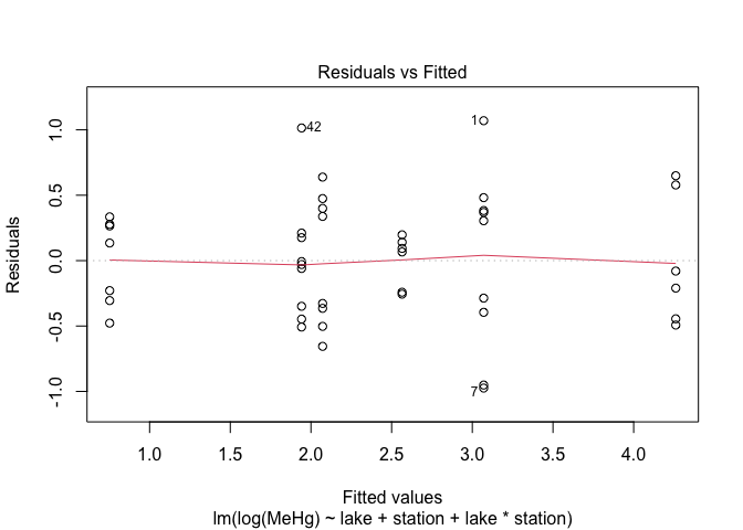
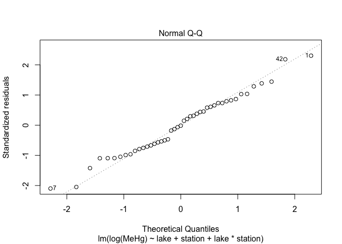 The assumptions of variance homogeneity and normality of residuals are satisfied
8.4 Interpretation of the interaction coefficient
# Example with two independent categorical variables
summary(mod4)
##
## Call:
## lm(formula = log(MeHg) ~ lake + station + lake * station, data = workshop)
##
## Residuals:
##      Min       1Q   Median       3Q      Max
## -0.97448 -0.34909 -0.00721  0.33475  1.06970
##
## Coefficients:
##                   Estimate Std. Error t value Pr(>|t|)
## (Intercept)         3.0705     0.1641  18.708  < 2e-16 ***
## lakeCSL2           -0.9982     0.2393  -4.172 0.000163 ***
## lakeCSL5           -0.5056     0.2595  -1.948 0.058588 .
## station2            1.1904     0.2595   4.587 4.56e-05 ***
## lakeCSL2:station2  -2.5101     0.3637  -6.901 2.93e-08 ***
## lakeCSL5:station2  -1.8133     0.3670  -4.941 1.51e-05 ***
## ---
## Signif. codes:  0 '***' 0.001 '**' 0.01 '*' 0.05 '.' 0.1 ' ' 1
##
## Residual standard error: 0.4924 on 39 degrees of freedom
## Multiple R-squared:  0.8317,	Adjusted R-squared:  0.8101
## F-statistic: 38.55 on 5 and 39 DF,  p-value: 4.427e-14
In the present example with 2 categorical variables, the interpretation as following:
1) lake AB35 and station 1 have been used as reference sites (control) to compare with other lakes and site. The concentration of MeHg at the reference site (station 1 in lake AB35) is 3.07 ng/g in periphyton. This is our baseline;

2) lakeCSL2 : MeHg concentration at sation 1 in lake CSL2 is about 1 ng/g less than station 1 in lake AB35,
   lakeCSL5 : MeHg concentration at sation 1 in lake CSL5 is about 0.5 ng/g less than station 1 in lake AB35;

3) station2 : MeHg concentration at sation 2 in lake AB35 is about 1.2 ng/g higher than station 1 in lake AB35;

4) lakeCSL2:station2 : MeHg concentration at station 2 in lake CSL2 is 2.5 ng/g less than station 2 in lake AB35.
   lakeCSL5:station2 : same as above for station 2 in lake CSL5.
There are 6 different cases of interpretation for multiple linear models with two independent variables, depending on the type of the independent variables, either continuous or categorical
1) Interaction between two categorical variables
2) Interaction between two continuous variables
3) Interaction between a categorical variable and a continuous variable
4) No interaction between two categorical variables
5) No interaction between two continuous variables
6) No interaction between a categorical variable and a continuous variable
To better understand the interpretation of output of lm(), I invite you to consult https://biologyforfun.wordpress.com/2014/04/08/interpreting-interaction-coefficient-in-r-part1-lm/
8.5 Post-hoc comparison
Careful!!
TukeyHSD() works only for aov(), not for lm(), and it is recommended not to use this function for 2-way ANOVA, because of type II error (False negative).
I highly recommend emmeans package for post-hoc comparison for 2-way ANOVA, easy to manipulate with more optional demands in the function emmeans().
res.2way5.emm<- emmeans(mod4,  pairwise ~ lake | station,adjust ="holm")
res.2way5.emm$contrasts %>% rbind()  %>% summary(infer = TRUE) # p-value adjust for 6
##  station contrast    estimate    SE df lower.CL upper.CL t.ratio p.value
##  1       AB35 - CSL2    0.998 0.239 39    0.333    1.663   4.172  0.0010
##  1       AB35 - CSL5    0.506 0.260 39   -0.216    1.227   1.948  0.3515
##  1       CSL2 - CSL5   -0.493 0.266 39   -1.232    0.247  -1.852  0.4293
##  2       AB35 - CSL2    3.508 0.274 39    2.747    4.270  12.807  <.0001
##  2       AB35 - CSL5    2.319 0.260 39    1.598    3.040   8.936  <.0001
##  2       CSL2 - CSL5   -1.189 0.248 39   -1.879   -0.500  -4.793  0.0001
##
## Results are given on the log (not the response) scale.
## Confidence level used: 0.95
## Conf-level adjustment: bonferroni method for 6 estimates
## P value adjustment: bonferroni method for 6 tests
res.2way5.emm$contrasts %>% summary(infer = TRUE) # p-value adjust for 3 in subgroups
## station = 1:
##  contrast    estimate    SE df lower.CL upper.CL t.ratio p.value
##  AB35 - CSL2    0.998 0.239 39    0.400    1.597   4.172  0.0005
##  AB35 - CSL5    0.506 0.260 39   -0.144    1.155   1.948  0.1172
##  CSL2 - CSL5   -0.493 0.266 39   -1.158    0.173  -1.852  0.1172
##
## station = 2:
##  contrast    estimate    SE df lower.CL upper.CL t.ratio p.value
##  AB35 - CSL2    3.508 0.274 39    2.823    4.194  12.807  <.0001
##  AB35 - CSL5    2.319 0.260 39    1.670    2.968   8.936  <.0001
##  CSL2 - CSL5   -1.189 0.248 39   -1.810   -0.569  -4.793  <.0001
##
## Results are given on the log (not the response) scale.
## Confidence level used: 0.95
## Conf-level adjustment: bonferroni method for 3 estimates
## P value adjustment: holm method for 3 tests
As mentioned, the adjustment of p-values depends on the objective of your studies. The adjustment of p-value can be done only for subgroups if your focus is to compare in subgroups. Otherwise, it is recommended to adjust for all p-values with the code showed above.
Section 3: Exercises
Context
Survey of trace metals concentrations in the water column in 3 different locations in 2004 and 2005 (56 observations and 7 variables)
# Description of data :
exercices<-read.csv('CEAEQ.csv')
View(exercices)
str(exercices)
1. Compute one-way anova with an independent factor (example of category)
# To study the effect of location on the concentration of Hg.
# Linear analysis with 1 categorical variable,
exe<-lm(Hg ~ lieu, data = exercices)
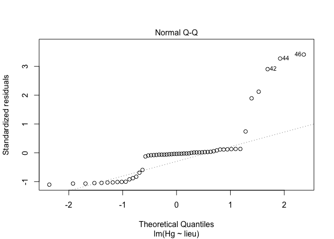
2. Verify the normality of the data, and choose the right data transformation
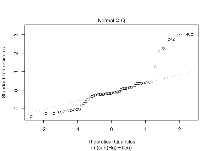
exe1<-lm(sqrt(Hg) ~ lieu, data = exercices) # square root transformation
exe2<-lm(log(Hg) ~ lieu, data = exercices) # log transformation
plot(exe,2)
plot(exe1,2)
plot(exe2,2)

summary(exe2)
##
## Call:
## lm(formula = log(Hg) ~ lieu, data = exercices)
##
## Residuals:
##     Min      1Q  Median      3Q     Max
## -2.1773 -0.8564 -0.2777  0.7660  2.5231
##
## Coefficients:
##             Estimate Std. Error t value Pr(>|t|)
## (Intercept)  -1.4371     0.3710  -3.874 0.000307 ***
## lieuLSL       1.2064     0.4507   2.677 0.009976 **
## lieuLSP-IS   -1.0096     0.4857  -2.079 0.042710 *
## lieuPM       -0.4501     0.5246  -0.858 0.394906
## ---
## Signif. codes:  0 '***' 0.001 '**' 0.01 '*' 0.05 '.' 0.1 ' ' 1
##
## Residual standard error: 1.173 on 51 degrees of freedom
##   (1 observation deleted due to missingness)
## Multiple R-squared:  0.3961,	Adjusted R-squared:  0.3606
## F-statistic: 11.15 on 3 and 51 DF,  p-value: 9.699e-06
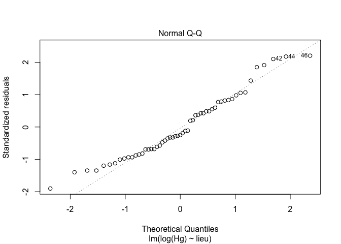 Conclusion : log transformation is good for this exercice
3. Pairwaise comparison with emmeans package
exe2.emm <- emmeans(exe2,  pairwise ~ lieu, adjust ="holm")
exe2.emm$contrasts %>% summary(infer = TRUE) %>% as.data.frame()
##         contrast   estimate        SE df   lower.CL   upper.CL    t.ratio
## 1      LSF - LSL -1.2064484 0.4507337 51 -2.4437493 0.03085252 -2.6766321
## 2 LSF - (LSP-IS)  1.0095951 0.4857250 51 -0.3237597 2.34294993  2.0785323
## 3       LSF - PM  0.4501440 0.5246430 51 -0.9900438 1.89033182  0.8580007
## 4 LSL - (LSP-IS)  2.2160435 0.4047708 51  1.1049145 3.32717251  5.4748101
## 5       LSL - PM  1.6565924 0.4507337 51  0.4192915 2.89389330  3.6753238
## 6  (LSP-IS) - PM -0.5594511 0.4857250 51 -1.8928059 0.77390370 -1.1517857
##        p.value
## 1 3.990514e-02
## 2 1.281299e-01
## 3 5.095601e-01
## 4 8.077295e-06
## 5 2.854498e-03
## 6 5.095601e-01
4. Compute a two-way anova
Study the effects of year and location on Hg concentrations
Example with two categorical factors
# Change data ownership
exercices$annee<-as.factor(exercices$annee)
exe3<-lm(log(Hg) ~ lieu + annee + lieu*annee, data = exercices)
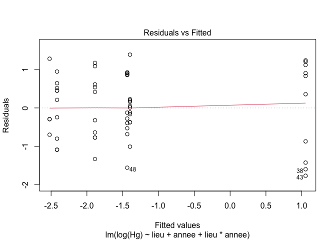
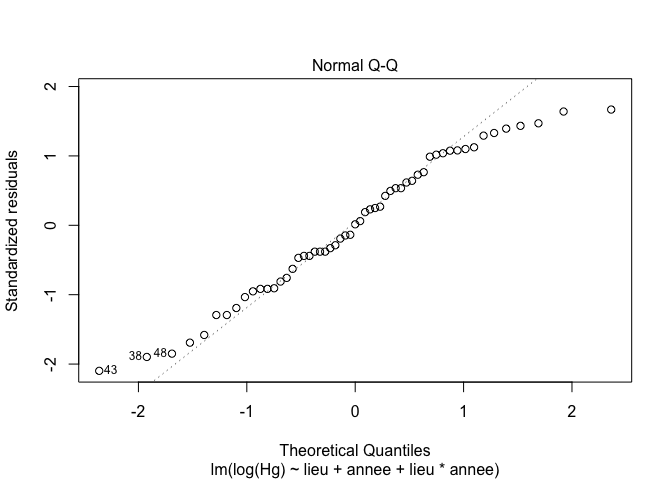
5. Checking assumptions
plot(exe3,1) # Look at the homogeneity of variances
plot(exe3,2) # Look at the normality of residuals
6. Models selection
exe4<-lm(log(Hg) ~ lieu + annee + lieu*annee, data = exercices) # with interaction
exe4.1<-lm(log(Hg) ~ lieu + annee, data = exercices) # additive effect
exe4.2<-lm(log(Hg) ~ lieu, data = exercices) # station effect
exe4.3<-lm(log(Hg) ~ annee, data = exercices) # years effect
AIC(exe4, exe4.1, exe4.2, exe4.3)
##        df      AIC
## exe4    7 150.6829
## exe4.1  6 161.5605
## exe4.2  5 179.4953
## exe4.3  3 198.4836
Conclusion : model with interaction has the smallest AIC value and should be selected as the best model to represent the relationship between the two factors and the response variable
Normally, when the different between tow AIC value < 2, we consider those two models are the same (which there is no case in this exercice). In this case, we chose the model with the less degree of freedom (df).
7. Interpreting output of analysis of variance
summary(exe4)
##
## Call:
## lm(formula = log(Hg) ~ lieu + annee + lieu * annee, data = exercices)
##
## Residuals:
##      Min       1Q   Median       3Q      Max
## -1.76739 -0.66087  0.01217  0.73901  1.38841
##
## Coefficients: (2 not defined because of singularities)
##                      Estimate Std. Error t value Pr(>|t|)
## (Intercept)           -1.5410     0.5958  -2.586 0.012718 *
## lieuLSL                0.1425     0.6532   0.218 0.828175
## lieuLSP-IS            -0.9799     0.3972  -2.467 0.017166 *
## lieuPM                -0.3462     0.6587  -0.526 0.601533
## annee2005              0.1039     0.5254   0.198 0.844004
## lieuLSL:annee2005      2.3486     0.6532   3.595 0.000751 ***
## lieuLSP-IS:annee2005       NA         NA      NA       NA
## lieuPM:annee2005           NA         NA      NA       NA
## ---
## Signif. codes:  0 '***' 0.001 '**' 0.01 '*' 0.05 '.' 0.1 ' ' 1
##
## Residual standard error: 0.8882 on 49 degrees of freedom
##   (1 observation deleted due to missingness)
## Multiple R-squared:  0.6675,	Adjusted R-squared:  0.6335
## F-statistic: 19.67 on 5 and 49 DF,  p-value: 1.064e-10
8. Pairwise comparison
exe4.2way5.emm<- emmeans(exe4,  pairwise ~ lieu | annee,adjust ="holm")
exe4.2way5.emm$contrasts %>% rbind()  %>% summary(infer = TRUE)
##  annee contrast       estimate    SE df lower.CL upper.CL t.ratio p.value
##  2004  LSF - LSL        nonEst    NA NA       NA       NA      NA      NA
##  2004  LSF - (LSP-IS)   nonEst    NA NA       NA       NA      NA      NA
##  2004  LSF - PM         nonEst    NA NA       NA       NA      NA      NA
##  2004  LSL - (LSP-IS)    1.122 0.519 49   -0.436    2.681   2.164  0.4239
##  2004  LSL - PM          0.489 0.388 49   -0.678    1.655   1.259  1.0000
##  2004  (LSP-IS) - PM    -0.634 0.525 49   -2.213    0.946  -1.206  1.0000
##  2005  LSF - LSL        -2.491 0.397 49   -3.685   -1.297  -6.272  <.0001
##  2005  LSF - (LSP-IS)    0.980 0.397 49   -0.214    2.174   2.467  0.2060
##  2005  LSF - PM         nonEst    NA NA       NA       NA      NA      NA
##  2005  LSL - (LSP-IS)    3.471 0.397 49    2.277    4.665   8.739  <.0001
##  2005  LSL - PM         nonEst    NA NA       NA       NA      NA      NA
##  2005  (LSP-IS) - PM    nonEst    NA NA       NA       NA      NA      NA
##
## Results are given on the log (not the response) scale.
## Confidence level used: 0.95
## Conf-level adjustment: bonferroni method for 12 estimates
## P value adjustment: bonferroni method for 12 tests
NB : NA in the output means no value to compare (i.e., in some years, there was no sampling in some locations)