Advanced data manipulation with tidyr and its allies
Jim Félix-Faure
October 2020
- Change table format
- Split two values from one cell
- Data set connection
- Manipulation of NA
- Practice
- Useful links
Note : To follow this workshop it is recommended to have already completed the following courses Fast data manipulation with dplyr and its allies and Rapid data visualization with ggplot2 (available on the Numerilab website - see link at the bottom of this document) or to have some basics on the use of the pipe operator, ggplot2 and the basic functions of the tidyverse.
Change table format
To optimize processing and/or visualization, it is recommended that the data tables under R be organized as follows :
- Each column is a variable..
- Each row is an observation.
- Each cell is composed of one value.
Let’s see some examples where this is not the case, and the solutions to apply using the tidyr package, included with the tidyverse.
From wide format to longer format
Here is an example where values are hidden in column names.
The weight of observations A and B is reported according to the year.
library(tidyverse)
Tbl_Weight <- tibble(
  Observation = c("A", "B"),
  "2010" = c(3, 3),
  "2011" = c(5, 2),
  "2012" = c(4, 3),
  "2013" = c(5, 3)
)
Tbl_Weight
# A tibble: 2 x 5
  Observation `2010` `2011` `2012` `2013`
  <chr>        <dbl>  <dbl>  <dbl>  <dbl>
1 A                3      5      4      5
2 B                3      2      3      3
How to compute the average weight of each observation? How to draw a graph representing the weight of each observation over time?
Not so easy, unless you reorganize the data. Here the objective is twofold:
- create a variable
Yeargrouping the years present in the name of the columns. - create a variable
Weightgrouping the weight values keeping the correspondence with the years.
Tbl_WeightTidy <- Tbl_Weight %>%
  pivot_longer(
    cols = !Observation, # Columns to be used
    names_to = "Year", # Variable where the column names will be stored
    names_transform = list(Year = as.integer), # Choice of variable type for names_to
    values_to = "Weight" # Variable where the values will be stored
  )
Tbl_WeightTidy
# A tibble: 8 x 3
  Observation  Year Weight
  <chr>       <int>  <dbl>
1 A            2010      3
2 A            2011      5
3 A            2012      4
4 A            2013      5
5 B            2010      3
6 B            2011      2
7 B            2012      3
8 B            2013      3
The average weight of observations :
Tbl_WeightTidy %>%
  group_by(Observation) %>%
  summarise(Mean = mean(Weight),
            Sd = sd(Weight),
            n = n())
`summarise()` ungrouping output (override with `.groups` argument)
# A tibble: 2 x 4
  Observation  Mean    Sd     n
  <chr>       <dbl> <dbl> <int>
1 A            4.25 0.957     4
2 B            2.75 0.5       4
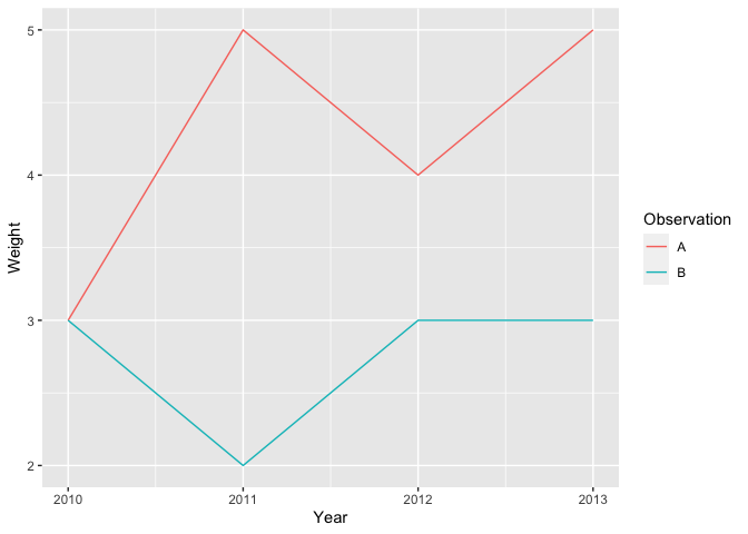
Graph of weights as a function of years :
Tbl_WeightTidy %>%
  ggplot() +
  geom_line(aes(x = Year, y = Weight, color = Observation))
From large format to wider format
Sometimes the problem is reversed. One observation is present in several rows and several variables are in the same column.
Tbl_Water <- tibble(
  Observation = rep(c("A", "B", "C", "D"), each = 2),
  Measure = rep(c("pH", "O2"), 4),
  Value = c(6, 99, 7, 90, 7.2, 85, 6.5, 96)
)
Tbl_Water
# A tibble: 8 x 3
  Observation Measure Value
  <chr>       <chr>   <dbl>
1 A           pH        6
2 A           O2       99
3 B           pH        7
4 B           O2       90
5 C           pH        7.2
6 C           O2       85
7 D           pH        6.5
8 D           O2       96
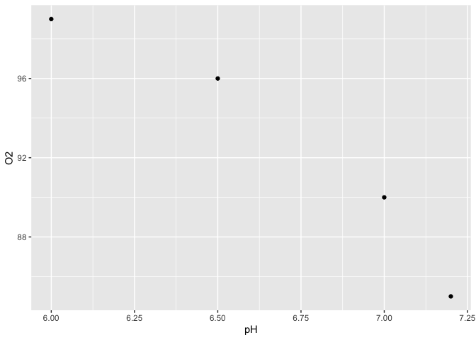
Again, it is not easy to graph the relationship between pH and O2 and the units in the Value column are not clear.
Tbl_WaterTidy <- Tbl_Water %>%
  pivot_wider(names_from = Measure, # column that contains the variable names
              values_from = Value # column that contains the values
              )
Tbl_WaterTidy
# A tibble: 4 x 3
  Observation    pH    O2
  <chr>       <dbl> <dbl>
1 A             6      99
2 B             7      90
3 C             7.2    85
4 D             6.5    96
Tbl_WaterTidy %>%
  ggplot(aes(x = pH, y = O2)) +
  geom_point()
Split two values from one cell
When entering data, it can happen that two values are put together in the same cell.
For example, here are the results of the number of animals positive to a molecule on the number of animals tested.
Tbl_Effect <- tibble(
  Molecule = c("A","B","C"),
  Result = c("87/112","23/48","34/89")
)
Tbl_Effect
# A tibble: 3 x 2
  Molecule Result
  <chr>    <chr>
1 A        87/112
2 B        23/48
3 C        34/89
We want to calculate the ratio between positive and tested animals.
The separate() function allows you to split the contents of one character column into several other character or numeric columns. It cuts out every character that is neither a number nor a letter. If necessary, the separator can be specified manually with the argument sep="".
Tbl_Effect %>%
  separate(
    col = Result, # which column to separate
    into = c("Positive_animals", "Tested_animals"), # how to call the new columns
    convert = TRUE, # convert the new columns to the appropriate type
    remove = TRUE # remove the former column
  ) %>%
  mutate(Ratio = Positive_animals/Tested_animals)
# A tibble: 3 x 4
  Molecule Positive_animals Tested_animals Ratio
  <chr>               <int>          <int> <dbl>
1 A                      87            112 0.777
2 B                      23             48 0.479
3 C                      34             89 0.382
Data set connection
The joins
As the number, source, and diversity of the data increase, it is common to have multiple data tables. In this case, it is possible to connect them using a key. Its nature can vary (character, factor, numeric…) but it is essential that this key be a unique value for each observation.
Let’s take a look at an example:
Tbl_Site <- tibble(
  Site = c("356a", "da4b", "77de", "1b64"),
  Landuse = c("Forest", "Forest", "Pasture", "Wetland"),
  Area = c(12, 30, 8, 17)
)
Tbl_Site
# A tibble: 4 x 3
  Site  Landuse  Area
  <chr> <chr>   <dbl>
1 356a  Forest     12
2 da4b  Forest     30
3 77de  Pasture     8
4 1b64  Wetland    17
Tbl_Result <- tibble(
  Site = c("1b64", "1b64", "356a", "da4b", "da4b", "abcd"),
  Measure = c("pH", "pH", "Corg", "pH", "Corg", "Corg"),
  Value = c(7, 7.2, 3.5, 5.8, 2.7, 5.8)
)
Tbl_Result
# A tibble: 6 x 3
  Site  Measure Value
  <chr> <chr>   <dbl>
1 1b64  pH        7
2 1b64  pH        7.2
3 356a  Corg      3.5
4 da4b  pH        5.8
5 da4b  Corg      2.7
6 abcd  Corg      5.8
As see below, there are many functions for joining data tables.
Full joins
The full_join() function allows to make a full join between two arrays. It will keep all the data of each table, at the risk of creating gaps (NA) when some information is not present in one or the other table.
full_join(Tbl_Site, Tbl_Result, by = "Site")
# A tibble: 7 x 5
  Site  Landuse  Area Measure Value
  <chr> <chr>   <dbl> <chr>   <dbl>
1 356a  Forest     12 Corg      3.5
2 da4b  Forest     30 pH        5.8
3 da4b  Forest     30 Corg      2.7
4 77de  Pasture     8 <NA>     NA
5 1b64  Wetland    17 pH        7
6 1b64  Wetland    17 pH        7.2
7 abcd  <NA>       NA Corg      5.8
The by= argument is used to specify on which variable to join. In our example, Site is used as the common key to both arrays.
Left joins
The left_join() function makes a left join. Which means on x, the table on the left. It will keep all the data from x and add the data from the right table (y) without incorporating data that does not match.
left_join(Tbl_Site, Tbl_Result, by = "Site")
# A tibble: 6 x 5
  Site  Landuse  Area Measure Value
  <chr> <chr>   <dbl> <chr>   <dbl>
1 356a  Forest     12 Corg      3.5
2 da4b  Forest     30 pH        5.8
3 da4b  Forest     30 Corg      2.7
4 77de  Pasture     8 <NA>     NA
5 1b64  Wetland    17 pH        7
6 1b64  Wetland    17 pH        7.2
Note that the new table does not contain the abcd site, not present in x (Tbl_Site).
Right joins
In the same way the right_join() function makes a right join (on y).
right_join(Tbl_Site, Tbl_Result, by = "Site")
# A tibble: 6 x 5
  Site  Landuse  Area Measure Value
  <chr> <chr>   <dbl> <chr>   <dbl>
1 356a  Forest     12 Corg      3.5
2 da4b  Forest     30 pH        5.8
3 da4b  Forest     30 Corg      2.7
4 1b64  Wetland    17 pH        7
5 1b64  Wetland    17 pH        7.2
6 abcd  <NA>       NA Corg      5.8
Note that the new table does not contain the 77de site, not present in y (Tbl_Result).
Filtering joins
The semi_join and anti_join functions allow to filter data table according to another.
semi_join will return all lines in x for which there is a match in y. Only the columns of x will be returned.
semi_join(Tbl_Site, Tbl_Result, by = "Site")
# A tibble: 3 x 3
  Site  Landuse  Area
  <chr> <chr>   <dbl>
1 356a  Forest     12
2 da4b  Forest     30
3 1b64  Wetland    17
In contrast, anti_join will return all lines in x for which there is no match in y. Only the columns of x will be returned.
anti_join(Tbl_Site, Tbl_Result, by = "Site")
# A tibble: 1 x 3
  Site  Landuse  Area
  <chr> <chr>   <dbl>
1 77de  Pasture     8
Bind data table
When the structure of the data tables is similar, it is sometimes preferable to bind these tables to form a single one.
In this example, we will use land-use data collected in 1970 and 2020 on the same site. In 2020, the areas of each site have been added.
Tbl_Site1970 <- tibble(
  Site = c("356a", "da4b", "77de", "1b64"),
  Landuse = c("Crop", "Pasture", "Pasture", "Wetland")
)
Tbl_Site2020 <- tibble(
  Site = c("356a", "da4b", "77de", "1b64"),
  Landuse = c("Forest", "Forest", "Pasture", "Crop"),
  Area = c(12, 30, 8, 17)
)
Tbl_Site1970
# A tibble: 4 x 2
  Site  Landuse
  <chr> <chr>
1 356a  Crop
2 da4b  Pasture
3 77de  Pasture
4 1b64  Wetland
Tbl_Site2020
# A tibble: 4 x 3
  Site  Landuse  Area
  <chr> <chr>   <dbl>
1 356a  Forest     12
2 da4b  Forest     30
3 77de  Pasture     8
4 1b64  Crop       17
There are two ways to do this:
By columns
With bind_cols, the y table is inserted to the right of the x table. The number of rows in x and y must be the identical. If column names are repeated the function adds a number behind the column name of y.
In most cases, a join is preferable…
bind_cols(Tbl_Site1970, Tbl_Site2020)
New names:
* Site -> Site...1
* Landuse -> Landuse...2
* Site -> Site...3
* Landuse -> Landuse...4
# A tibble: 4 x 5
  Site...1 Landuse...2 Site...3 Landuse...4  Area
  <chr>    <chr>       <chr>    <chr>       <dbl>
1 356a     Crop        356a     Forest         12
2 da4b     Pasture     da4b     Forest         30
3 77de     Pasture     77de     Pasture         8
4 1b64     Wetland     1b64     Crop           17
Sometimes it is useful to extract a variable from a data table without importing the initial table:
bind_cols(Tbl_Site1970, select(Tbl_Site2020, Area))
# A tibble: 4 x 3
  Site  Landuse  Area
  <chr> <chr>   <dbl>
1 356a  Crop       12
2 da4b  Pasture    30
3 77de  Pasture     8
4 1b64  Wetland    17
Warning: Both tables must be ordered in the same way.
By rows
With bind_rows, the y table is inserted under the x table.
bind_rows(Tbl_Site1970, Tbl_Site2020)
# A tibble: 8 x 3
  Site  Landuse  Area
  <chr> <chr>   <dbl>
1 356a  Crop       NA
2 da4b  Pasture    NA
3 77de  Pasture    NA
4 1b64  Wetland    NA
5 356a  Forest     12
6 da4b  Forest     30
7 77de  Pasture     8
8 1b64  Crop       17
Note that not all columns need to be present in both tables. In this case, NAs are generated.
The argument .id is used to identify which table the data comes from by creating a new column containing the id. It is possible to choose the name of the column containing the id and the identifier of each table.
bind_rows("1970" = Tbl_Site1970, "2020" = Tbl_Site2020, .id = "Year")
# A tibble: 8 x 4
  Year  Site  Landuse  Area
  <chr> <chr> <chr>   <dbl>
1 1970  356a  Crop       NA
2 1970  da4b  Pasture    NA
3 1970  77de  Pasture    NA
4 1970  1b64  Wetland    NA
5 2020  356a  Forest     12
6 2020  da4b  Forest     30
7 2020  77de  Pasture     8
8 2020  1b64  Crop       17
Manipulation of NA
In a data table, missing values (NA) are often a source of problems and difficulties.
To avoid problems, some machines use a specific code to signify missing or outlier data, for example 9999 or -9999. Sometimes it is when entering our data that we use a code, for example "NoData".
In a case like this, to perform analyses we may want to:
Convert values to NA.
The function na_if(x, y) is used to convert the values y contained in x to NA.
Here is an example:
Tbl_Temperature <- tibble(Site = c("A", "A", "A", "B", "B", "B"),
             Month = c("January", "NoData", "September", "January", "June", "September"),
             Temp = c(-12, 16, 13, 9999, 19, 15 ))
Tbl_Temperature
# A tibble: 6 x 3
  Site  Month      Temp
  <chr> <chr>     <dbl>
1 A     January     -12
2 A     NoData       16
3 A     September    13
4 B     January    9999
5 B     June         19
6 B     September    15
One value is missing in the Month variable (NoData) and one value is identified as an outlier in the Temp variable. We then replace these two values by NA as follow:
Tbl_TempNA <- Tbl_Temperature %>%
  mutate(Month = na_if(Month, "NoData")) %>%
  mutate(Temp = na_if(Temp, 9999))
Tbl_TempNA
# A tibble: 6 x 3
  Site  Month      Temp
  <chr> <chr>     <dbl>
1 A     January     -12
2 A     <NA>         16
3 A     September    13
4 B     January      NA
5 B     June         19
6 B     September    15
Replace NA
The replace_na function allows you to replace the NA with one or more other values.
Tbl_TempNA
# A tibble: 6 x 3
  Site  Month      Temp
  <chr> <chr>     <dbl>
1 A     January     -12
2 A     <NA>         16
3 A     September    13
4 B     January      NA
5 B     June         19
6 B     September    15
Tbl_TempNA %>%
  mutate(Month = replace_na(Month, "June")) %>%
  mutate(Temp = replace_na(Temp, -17))
# A tibble: 6 x 3
  Site  Month      Temp
  <chr> <chr>     <dbl>
1 A     January     -12
2 A     June         16
3 A     September    13
4 B     January     -17
5 B     June         19
6 B     September    15
or :
Tbl_TempNA %>%
  replace_na(list(Month = "June", Temp = -17))
# A tibble: 6 x 3
  Site  Month      Temp
  <chr> <chr>     <dbl>
1 A     January     -12
2 A     June         16
3 A     September    13
4 B     January     -17
5 B     June         19
6 B     September    15
Practice
Table formatting
Transform the following data sets into a table ready for analysis, considering that the unit of observation is the season.
Tbl_Meteo consists of the average annual weather conditions.
Tbl_Weather <- tribble(
  ~State, ~Temp, ~Rain,
  "Quebec", 15, 300,
  "Ontario", 17, 280,
  "Manitoba", 12, 360
)
Tbl_Obs consists of wildlife observations (positive/total).
Tbl_Obs <- tribble(
  ~State, ~Spring, ~Fall,
  "Quebec", "22/30", "10/12",
  "Ontario", "18/50", "3/4"
)
The final table should look like this:
# A tibble: 4 x 6
  State    Temp  Rain Season Obs_posi Obs_nega
  <chr>   <dbl> <dbl> <chr>     <int>    <int>
1 Quebec     15   300 Spring       22        8
2 Quebec     15   300 Fall         10        2
3 Ontario    17   280 Spring       18       32
4 Ontario    17   280 Fall          3        1
Useful links
This workshop is largely inspired by free documents and website.
Thanks to Charles Martin PhD student at UQTR for his help.
Here are some useful links to continue:
Your favorite site:
- https://rive-numeri-lab.github.io/
Safe memory help for the tidyr package:
- https://tidyr.tidyverse.org/
More generally and to complete on the tidyverse:
- https://www.tidyverse.org/