Watershed Analysis
Jade Dormoy-Boulanger
February 2026
By the end of this workshop, you will be able to delineate a watershed using QGIS and extract land use data from it using R.
You will need this land use map (from Agriculture and Agri-Food Canada’s crop inventory) -> https://ouvert.canada.ca/data/fr/dataset/32546f7b-55c2-481e-b300-83fc16054b95
You will also need to create a free account and obtain an API key from OpenTopography -> https://opentopography.org/blog/introducing-api-keys-access-opentopography-global-datasets
To make sure you get the most out of this workshop, let’s start with a few theoretical concepts:
Theoretical Background
In this workshop, we will be working with two types of GIS (Geographic Information System) objects: vectors and rasters.
A vector is a geometric object defined by points and lines, based on mathematical coordinates. It is generally used to represent linear or bounded features, such as roads or boundaries. In our case, the watershed we will generate will be in vector format.
A raster, on the other hand, is essentially an image: a grid of pixels, where each pixel contains a piece of information. We will be using a land use map from Agriculture and Agri-Food Canada’s crop inventory, in which each pixel colour corresponds to a particular type of activity.
By overlaying these different GIS layers, it becomes possible to reconstruct a landscape and analyze the interactions between them, for example, between the boundaries of a watershed and its land use.
Additionally, every GIS object is associated with a georeferencing system. In practice, each geographic coordinate (latitude, longitude) is defined relative to a Spatial Reference System (SRS), which makes it possible to locate objects on a representation of the Earth, whether that’s a flat grid like a map, or an ellipsoid like a globe.
SRS differ notably in their unit of measurement: some express coordinates in meters (like the UTM system), others in degrees (like WGS84, also known as EPSG 4326). Since we won’t be calculating distances in this workshop, we will use the EPSG 4326 system.
QGIS
1 - Loading a Basemap
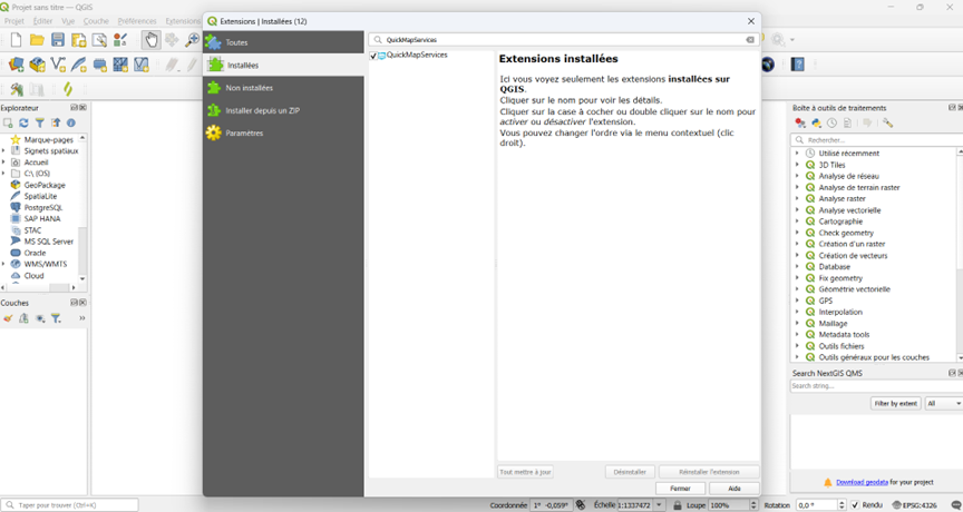
We will work with a Google Maps basemap. To do so, you need to install the QuickMapServices plugin:
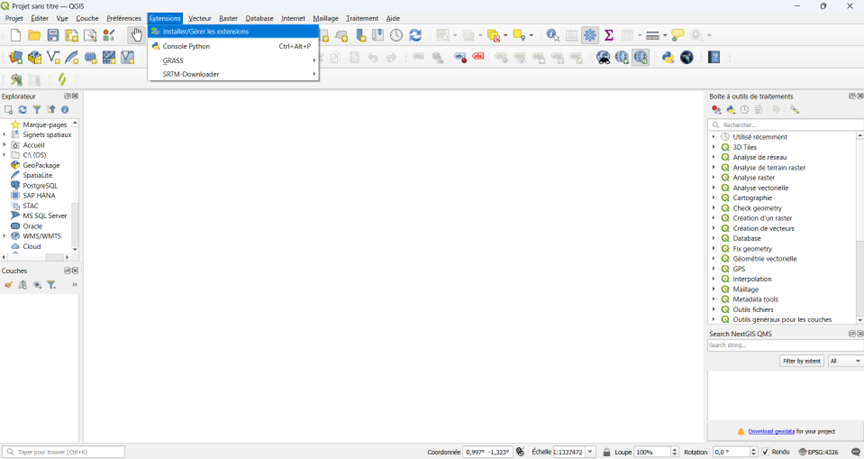
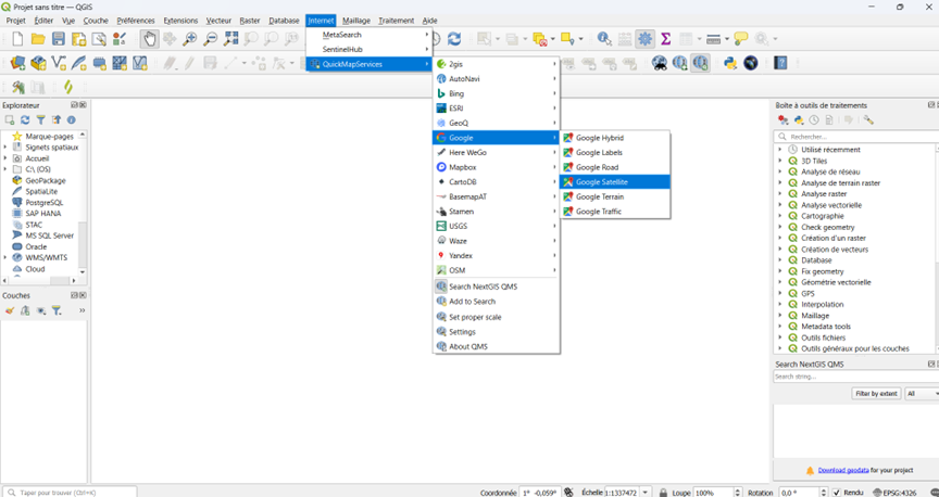
Then, display the Google Maps basemap:
Web tab -> QuickMapServices -> Google -> Google Satellite
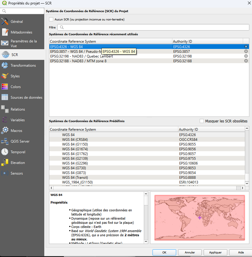
2 - Setting the SRS
We will change the SRS to EPSG 4326
3 - Downloading Elevation Data (DEM)
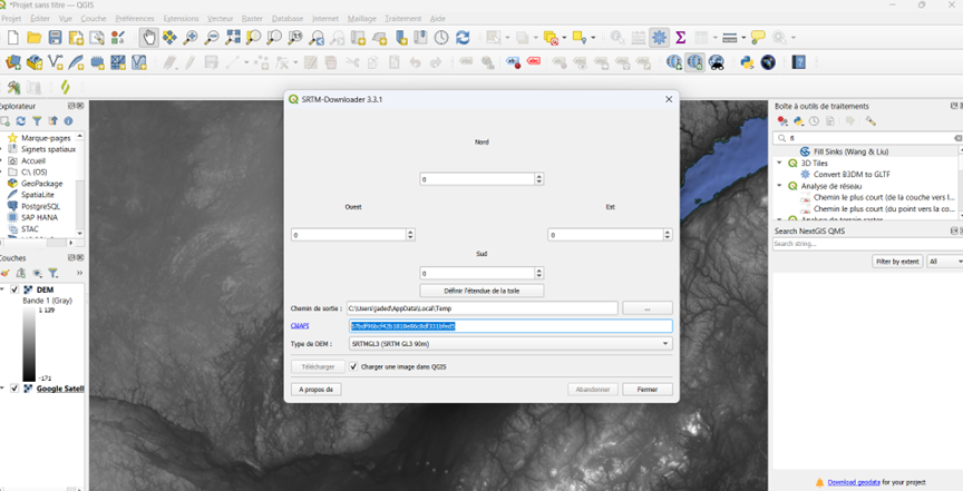
To calculate a watershed, you need elevation data for the area of interest. This data is available through SRTM satellites:
Install the SRTM-Downloader plugin
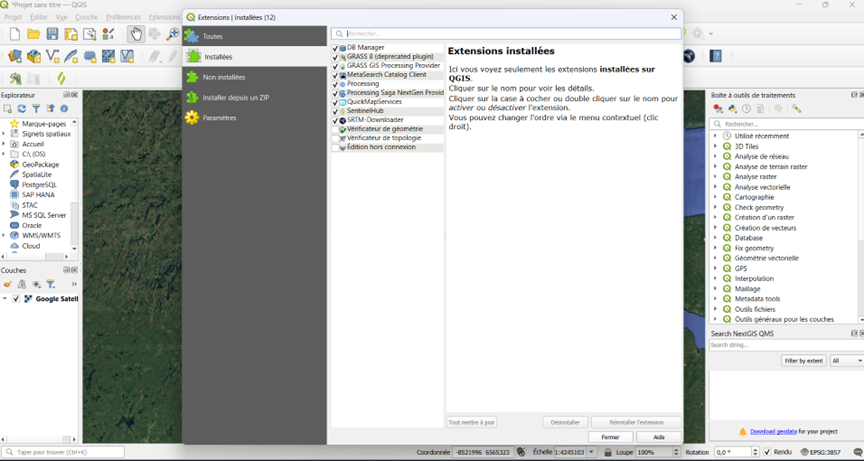
Plugins tab -> SRTM-Downloader
Click on Set canvas extent to define the dimensions of the elevation data, and enter the API key obtained from OpenTopography at the beginning of the workshop.
Click Download and then Close
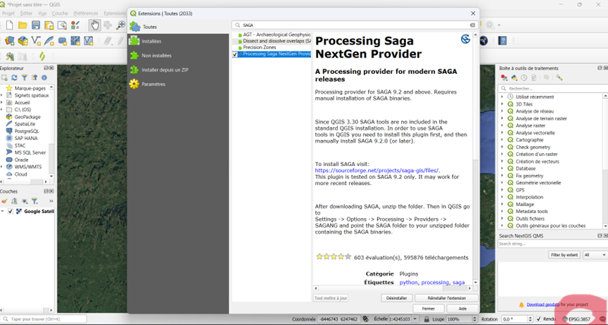
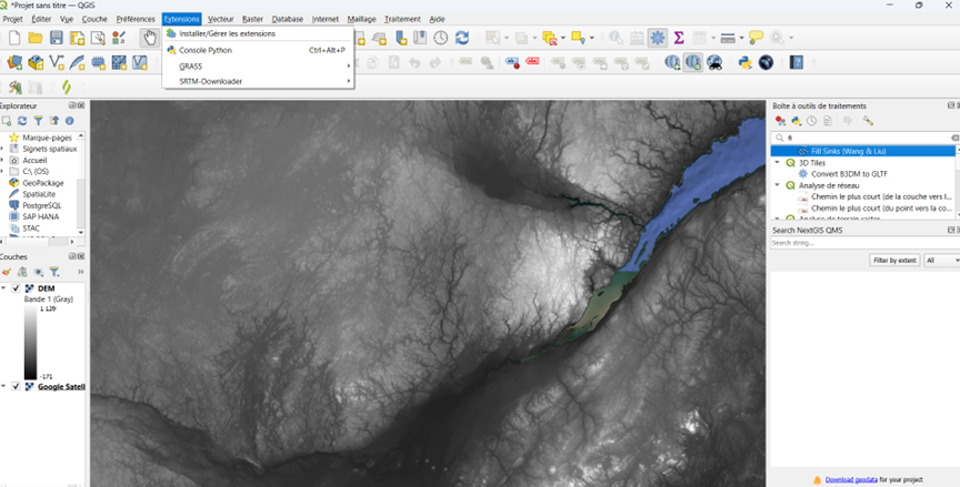
4 - Installing SAGA Tools
In the search bar of the Plugins tab, search for SAGA.
Install Processing Saga NextGen Provider
5 - Watershed Delineation
We will use the Fill sinks (Wang & Liu) algorithm to identify and fill depression areas in our elevation model. Make sure to select the SAGA version!
In the DEM field, enter the DEM [EPSG:4326], then click Run
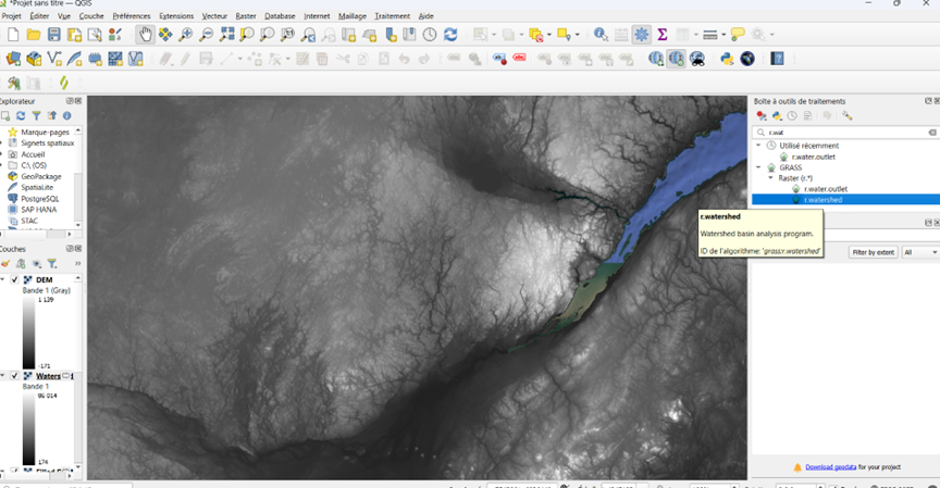
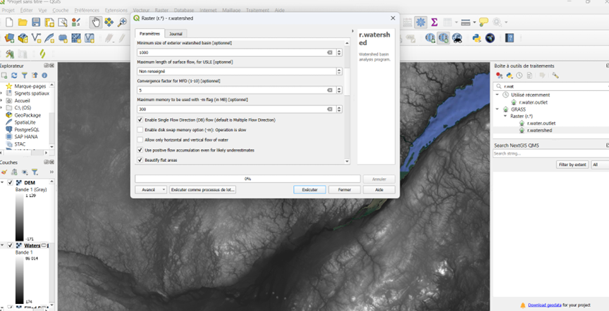
We will then compute the hydrological characteristics of the watersheds in the study area (flow direction, flow accumulation, stream networks, etc.) using the r.watershed tool from GRASS
In the Elevation menu, select Filled DEM [EPSG:4326]
In the Minimum size of exterior watershed basin field, enter 1000
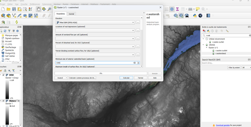
Check only Enable Single Flow, Use positive flow, and Beautify flat areas
Click Run then Close
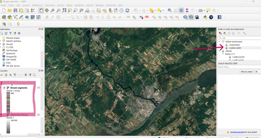
In the Layers panel at the bottom left, uncheck everything except Stream segments and Google Satellite
Find and open the r.water.outlet tool from GRASS
In the Drainage direction raster menu, select Drainage direction [EPSG:4326]
Click the three dots to the right of the Coordinates of outlet point field and click on the map at the location of your station.
Click Run and then Close
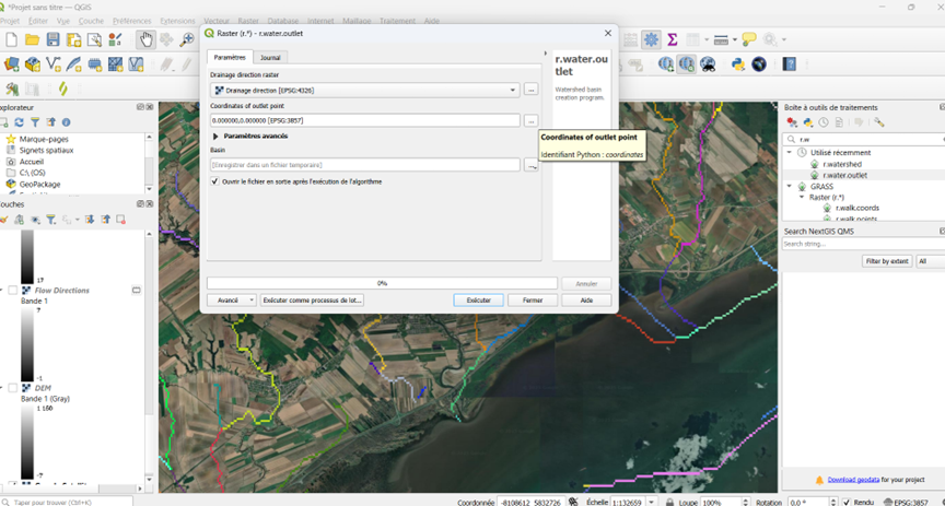
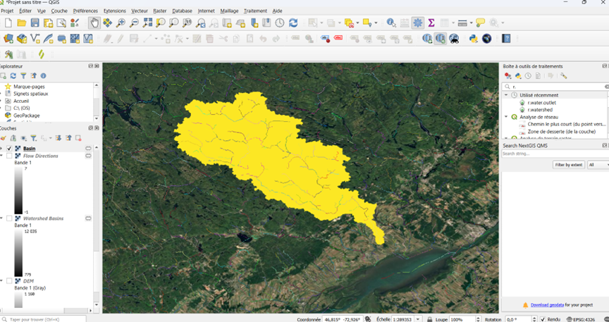
Your watershed should now appear on your map
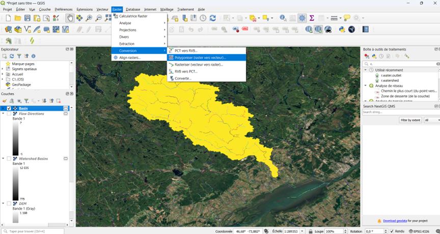
6 - Exporting the Watershed
To export the watershed, we first need to convert it to a vector format.
Raster tab -> Conversion -> Polygonize (raster to vector)
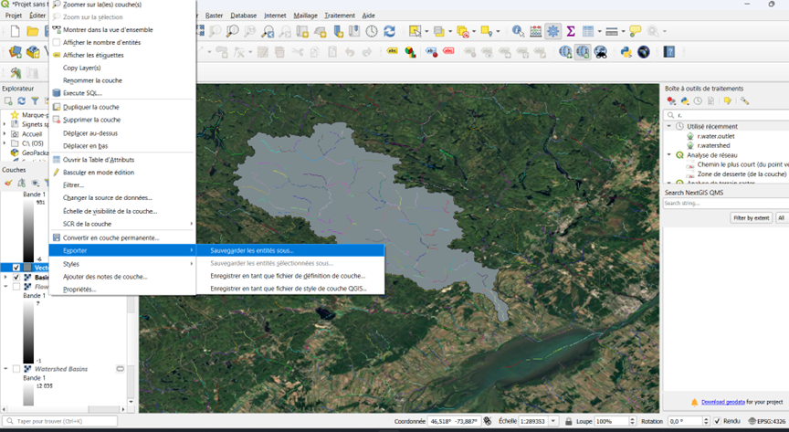
Then, right-click on the newly created vector layer -> Export -> Save Features As…
Select the ESRI Shapefile format
In the File name field, enter the desired name and click on the three dots to choose where the file will be saved
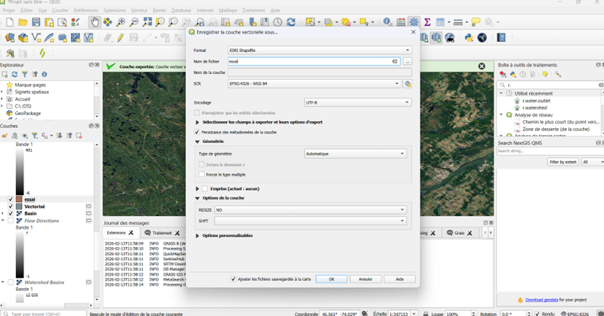
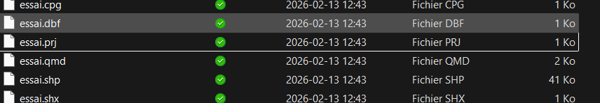
Heads up! The export will create 6 files. These 6 files make up your shapefile and must always be kept together!
7 - Extracting Land Use Data
Now that we have a watershed boundary in shapefile format, we can import it into R and use it to extract land use data. We will also need a land use raster. For this workshop, I used the 2020 Annual Crop Inventory from Agriculture and Agri-Food Canada, available here -> https://ouvert.canada.ca/data/fr/dataset/32546f7b-55c2-481e-b300-83fc16054b95
library(sf)
library(tmap)
library(terra)
library(tidyverse)

#Shapefile importation
essai <- st_read("essai.shp")
Reading layer `essai' from data source
  `/Users/charlesmartin/My Drive/UQTR_Pro/Numerilab/Ateliers/BassinsVersantsJade/essai.shp'
  using driver `ESRI Shapefile'
Simple feature collection with 2 features and 2 fields
Geometry type: POLYGON
Dimension:     XY
Bounding box:  xmin: -73.63875 ymin: 46.29458 xmax: -72.89042 ymax: 46.83875
Geodetic CRS:  WGS 84
#Everything worked!
tmap_mode("view")
tm_shape(essai) + tm_polygons()
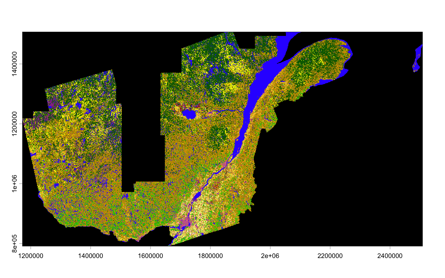
#Land use raster importation
landuse = rast("aci_2020_qc_v4.tif")

#Everything worked!
str(landuse)
S4 class 'SpatRaster' [package "terra"]
plot(landuse)
#Swiping numerical categories with their definition, as per Agriculture and #Agrifood Canada's guidelines

landuse_classes <-data.frame(lu_code = c(10,20,30,34,35,50,80,85,110,120,122,130:143,145:158, 160:163, 167,168,174:183, 185,188:200, 210,220,230),

landuse_class = c("Cloud", "Water","Exposed_Land_Barren", "Urban_Developed",
                                          "Greenhouses","Shrubland","Wetland","Peatland","Grassland",
                                          "Agriculture","Pasture_Forages","Too_Wet_to_be_Seeded",
                                          "Fallow","Cereals","Barley","Other_Grains","Millet","Oats","Rye",
                                          "Spelt","Triticale","Wheat","Switchgrass","Sorghun","Quinoa","Winter_Wheat",
                                          "Spring_Wheat","Corn","Tobacco","Ginseng","Oilseeds","Borage","Camelia",
                                          "Canola_Rapeseed","Flaxseed","Mustard","Safflower","Sunflower","Soybeans",
                                          "Pulses","Other_Pulses","Peas","Chickpeas","Beans","Fababeans","Lentils",
                                          "Vegetables","Tomatoes","Potatoes","Sugarbeets","Other Vegetables","Fruits",
                                          "Berries","Blueberry","Cranberry","Other Berry","Orchards","Other Fruits",
                                          "Vineyard","Hops","Sod","Herbs","Nursery","Buckwheat","Canaryseed","Hemp",
                                          "Vetch","Other_Crops","Forest","Coniferous","Broadleaf","Mixedwood"))

levels(landuse)<-landuse_classes
The next step is to convert our boundary shapefile into a SpatVector format and to reproject it under the same coordinate system as the land use map. Once compatible, we will be able to extract information on land use.
#Shapefile conversion into a compatible format
spoly = vect(essai) %>%
  terra::project(landuse)

#Land use data extraction
landuse.essai = landuse %>%
  terra::extract(spoly) %>%
  count(ID, landuse_class)
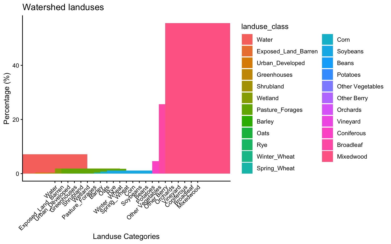
One last thing that might be interesting is to create a dataframe containing land use percentage. This way we could determine what is the predominant land use in our watershed.
#Pixels' number conversion into percentage, according to land use
landuse.essai<-mutate(landuse.essai,percent= (n*100)/sum(n))

#Quick visualisation graph
graph <- ggplot(landuse.essai) +
  geom_col(aes(x = landuse_class, y = percent, fill = landuse_class, width = 5))+
  theme_classic()+
  theme(axis.text.x = element_text(angle=45, hjust = 1))+
   xlab("Landuse Categories") +ylab("Percentage (%)")+
  ggtitle("Watershed landuses")

graph