Gentle transition to the Bayesian approach
Charles Martin
September 2025
- Introduction
- Review of the frequentist approach
- The Bayesian version
- The Markov Chain Monte Carlo method (MCMC)
- Integrating prior information
- Did my MCMC work well?
- Is my model good?
- Is this model better than another?
- Conclusion
Introduction
If you’re like me, Bayesian statistics have probably always seemed like an ideal. Something that others do, not you. They, the real statisticians!
The purpose of this workshop is to deconstruct this myth. To show you that in 2025, this approach is not only accessible but also easier to interpret and more direct. It’s actually everything you have always wanted your statistics to be! We will even manage the whole workshop without any mathematical equations!
The frequentist approach to statistics, i.e., the one you have been taught until now, is based on the principle that there is a fixed “true” value, the population value, for each of the parameters you want to estimate. The frequentist approach then provides you with a series of tools (T-test, ANOVA, etc.) that are designed so that, in the long run, if used a very large number of times, their statistical properties (p-value, confidence interval) will hold true.
From a Bayesian perspective, the uncertainty in our estimates, the probabilities themselves, are a consequence of our inability to measure everything in detail. Uncertainty is our tool to evaluate everything we don’t understand or can’t measure about a system. The data are therefore considered real and precise: this is what we have measured. The parameters, on the other hand, are the object of uncertainty. We cannot know the phenomenon precisely because we cannot measure everything.
The other fundamental aspect of the Bayesian approach is that it is designed as a process of knowledge update. Before the experiment, we have a certain amount of information and certainties. We then collect data, which allows us to update our knowledge about the phenomenon under study. This aspect is both the most powerful and the most polarizing of the Bayesian approach, as it allows, if needed, the introduction of some subjectivity in the process.
On the one hand, some will say that this subjectivity has no place in science and that each experiment should be viewed in isolation. But many will tell you that today, a large part of the replication problems faced by modern science could have been avoided if the analysis of the most outlandish (or innovative!) hypotheses had begun with a very low prior probability that the hypothesis was true.
Review of the frequentist approach
Before we dive into the Bayesian approach, let’s take a moment to review the frequentist approach. Here, we will try to answer the question: what influences the weight of penguins from the Palmer Archipelago? Among the phenomena of interest, we measured the length of the wings (mm, swimming ability), the length of the beak (mm, prey size), the sex, and the species of each individual. We will try to see how these variables influence the weight of the birds (g).
So, let’s start by loading the necessary libraries, namely tidyverse for data manipulation and visualization, and palmerpenguins for the data itself.
library(tidyverse)
library(palmerpenguins)
Next, let’s prepare a small data frame that will follow us throughout the exercise:
manchots <- penguins |>
  select(body_mass_g, flipper_length_mm, bill_length_mm, sex, species) |>
  drop_na()
By the way, note that the Bayesian approach would be perfectly suitable for imputing this missing data rather than simply eliminating it, but that’s a topic for another day…
Then, using the lm function, let’s fit a multiple regression model that will try to answer our question:
m <- lm(
  body_mass_g ~
    flipper_length_mm + bill_length_mm + sex + species,
  data = manchots
)
summary(m)
Call:
lm(formula = body_mass_g ~ flipper_length_mm + bill_length_mm +
    sex + species, data = manchots)

Residuals:
    Min      1Q  Median      3Q     Max
-718.50 -201.60  -12.75  198.45  878.24

Coefficients:
                  Estimate Std. Error t value Pr(>|t|)
(Intercept)       -759.064    541.377  -1.402 0.161834
flipper_length_mm   17.847      2.902   6.150 2.25e-09 ***
bill_length_mm      21.633      7.148   3.027 0.002670 ** sexmale            465.395     43.081  10.803  < 2e-16 ***
speciesChinstrap  -291.711     81.502  -3.579 0.000397 ***
speciesGentoo      707.028     94.359   7.493 6.35e-13 ***
---
Signif. codes:  0 '***' 0.001 '**' 0.01 '*' 0.05 '.' 0.1 ' ' 1

Residual standard error: 292 on 327 degrees of freedom
Multiple R-squared:  0.8705,    Adjusted R-squared:  0.8685
F-statistic: 439.7 on 5 and 327 DF,  p-value: < 2.2e-16
confint(m)
                         2.5 %     97.5 %
(Intercept)       -1824.084819  305.95606
flipper_length_mm    12.138156   23.55487
bill_length_mm        7.571439   35.69361
sexmale             380.644608  550.14539
speciesChinstrap   -452.044957 -131.37631
speciesGentoo       521.400228  892.65574
So, in short, penguin weight increases with wing length and beak size, males are heavier than females, and Chinstrap and Gentoo penguins are respectively lighter and heavier than Adelie (the reference level).
Where things get complicated is when we look at the details of the statistics. For example, try to state the frequentist definition of a confidence interval without looking it up online!
(pause)
It’s an interval of values that, if we repeat the sampling many times under the same conditions, will contain the true population value a certain percentage of the time (e.g., 95%).
For the effect of wing length, the interval is between 12.14 and 23.55 g per mm of wing. We would like to be able to say that there is a 95% chance that the true population value is between these bounds, but nothing in the frequentist approach allows us to do so. This philosophy assumes that the population value is fixed, and then it quantifies the error produced by the sampling process. The interpretation we commonly make (95% chance that the true value is within the interval) is a purely Bayesian interpretation of reality.
The other statistic that is commonly interpreted in these outputs is the p-value. Once again, can you recall the precise definition of a p-value from memory?
(pause)
The p-value is the probability of observing data at least as extreme as those found if the null hypothesis is true (here, that the parameter is exactly zero).
-
It is NOT the probability that the null hypothesis is true.
-
It is NOT the probability that the result is due to chance.
-
Above all, it tells us NOTHING about the magnitude or size of the effect.
If we work within a frequentist framework, our only inference tools are a confidence interval, based on the long term, which tells us nothing about the current data, and a p-value, which tells us about the probability of finding hypothetical data more extreme than those found if a fanciful hypothesis is true (i.e., the effect is exactly zero).
Let’s now see how things could unfold with the Bayesian approach.
The Bayesian version
The first thing to know is that there are now several R libraries that greatly facilitate the most common analyses in Bayesian mode. The rstanarm library is an excellent starting point as it contains equivalents for the most well-known modeling functions such as stan_lm, stan_aov, stan_glm, stan_glmer, stan_nlmer, and stan_gamm4. Moreover, its models are pre-compiled, which makes them almost as fast as the frequentist versions. In most cases, we are talking about a difference of just a few seconds.
So, let’s load this library, and then, let’s allow it to use multiple cores on our computer to speed up the treatments that can be done in parallel.
library(rstanarm)
Loading required package: Rcpp

This is rstanarm version 2.32.1

- See [https://mc-stan.org/rstanarm/articles/priors](https://mc-stan.org/rstanarm/articles/priors) for changes to default priors!

- Default priors may change, so it's safest to specify priors, even if equivalent to the defaults.

- For execution on a local, multicore CPU with excess RAM we recommend calling

  options(mc.cores = parallel::detectCores())
options(mc.cores = parallel::detectCores()-1)
Note that I am keeping one core (-1) so that my computer remains usable during processing. If this is not a priority for you, you can let it use all cores.
To defuse any tension, here is the same model immediately, analyzed within a Bayesian framework:
m_bayes <- stan_glm(
  body_mass_g ~
    flipper_length_mm + bill_length_mm + sex + species,
  data = manchots
)
summary(m_bayes)
Model Info:
 function:     stan_glm
 family:       gaussian [identity]
 formula:      body_mass_g ~ flipper_length_mm + bill_length_mm + sex + species
 algorithm:    sampling
 sample:       4000 (posterior sample size)
 priors:       see help('prior_summary')
 observations: 333
 predictors:   6

Estimates:
                    mean    sd      10%     50%     90%
(Intercept)        -748.7   548.4 -1451.0  -752.9   -53.7
flipper_length_mm    17.8     3.0    14.0    17.8    21.6
bill_length_mm       21.4     7.2    12.2    21.2    30.5
sexmale             466.3    42.9   411.4   466.0   520.9
speciesChinstrap   -289.3    82.0  -393.5  -288.7  -185.8
speciesGentoo       709.0    95.2   590.8   707.3   829.6
sigma               293.0    11.2   278.9   292.7   307.3

Fit Diagnostics:
           mean   sd     10%    50%    90%
mean_PPD 4206.9   22.9 4177.9 4206.9 4236.7

The mean_ppd is the sample average posterior predictive distribution of the outcome variable (for details see help('summary.stanreg')).

MCMC diagnostics
                  mcse Rhat n_eff
(Intercept)       12.2  1.0 2006
flipper_length_mm  0.1  1.0 2505
bill_length_mm     0.2  1.0 1963
sexmale            0.9  1.0 2086
speciesChinstrap   1.9  1.0 1840
speciesGentoo      2.3  1.0 1653
sigma              0.2  1.0 3246
mean_PPD           0.4  1.0 3875
log-posterior      0.0  1.0 1695

For each parameter, mcse is Monte Carlo standard error, n_eff is a crude measure of effective sample size, and Rhat is the potential scale reduction factor on split chains (at convergence Rhat=1).
posterior_interval(m_bayes)
                            5%        95%
(Intercept)       -1654.022655  143.67009
flipper_length_mm    13.005745   22.79919
bill_length_mm        9.675732   33.06481
sexmale             398.062553  537.16807
speciesChinstrap   -419.471533 -156.80500
speciesGentoo       554.227684  864.33638
sigma               275.195951  311.73817
That’s it, you have run your first Bayesian model! Everything is identical except for 4 characters (stan_).
First, note the reassuring thing: the average parameter estimates are essentially identical to those produced by lm. Among other things, the effect of wing length is 17.83 g/mm vs. 17.85 g/mm, males are 466.02 g heavier than females vs. 465.4 in the frequentist approach, etc.
Your figures for the Bayesian approach might be slightly different from mine, which is completely normal as it is a random sampling process.
The first advantage of the Bayesian approach is that we can directly interpret the uncertainty associated with the parameters. For example, the 95% credibility interval for the effect of wing length ranges from 13.01 and 22.8 g/mm. So, here, we are entitled to say that there is a 95% chance that the true value of the parameter is between these two bounds! No complicated definition, nothing about uncollected hypothetical samples. That’s all: 95% chance that the true effect of wing length is between 13.01 and 22.8 g/mm.
The Markov Chain Monte Carlo method (MCMC)
After this little bit of magic, it is obviously useful to explain how stan_glm arrived at these numbers.
You may know that there are several ways to find the best values for parameters in a statistical model.
The lm function uses a short sequence of matrix algebra to produce parameters that will always minimize the sum of the squared residuals.
In more complex cases such as GLMs or mixed models, the classical approach is rather to maximize the likelihood of the model. In other words, to find the most probable parameter values given the data. In this case, the algorithm starts from a random solution and moves through the likelihood landscape to try to find the most probable combination of values. If you have received non-convergence error messages in the past, it means that this algorithm has not managed to stabilize in one place. It oscillates without being able to determine the best combination.
In these two paradigms, the uncertainty around the parameters is then estimated from the variance/covariance matrix, with the assumption that this uncertainty follows a normal, symmetric distribution around the parameter.
The Bayesian approach is quite different. First, its exploration of the likelihood landscape is based on the Markov Chain Monte Carlo method (MCMC). This technique alone would deserve its own Numerilab workshop, but the main idea is as follows: from a point in the landscape, the Markov chain randomly determines a destination, and the more probable this destination is, the more likely it is to be explored. If the algorithm decides to explore this point, the probability of observing the data at that location is evaluated, and then it serves as the basis for the next jump. The main consequence of this way of doing things is that the more probable a location in the landscape is, the more often it will be explored.
Several algorithms have been proposed to perform this exploration, including the Metropolis-Hasting algorithm and then Gibbs sampling. But at present, THE way to do it is the NUTS (No U-Turn Sampling) algorithm, a variant of the Hamiltonian method, implemented in the specialized Stan programming language.
Behind the scenes, rstanarm also uses this programming language to fit your models. It simply translates your formulas and data definition into a format understandable by Stan, and then executes this code and retrieves the results.
Besides the method for traversing the landscape, the other main difference is that the MCMC method, rather than keeping only the final destination, will keep each step of the exploration. And since the MCMC explores the most probable places more densely, the distribution of the values explored by the chain will directly give us the probability distribution of the values that a parameter could take.
Each exploration step is called a draw from the Markov chain and is contained in the result object. These samples are already present in the m_bayes object. We just need to convert it into a data frame to proceed:
echantillons <- m_bayes |>
  as.data.frame() |>
  janitor::clean_names()
head(echantillons)
   intercept flipper_length_mm bill_length_mm  sexmale species_chinstrap
1  -573.9174          18.19149       15.80594 513.3798        -260.31328
2  -252.0096          16.18211       14.70172 504.1950         -83.48346
3  -946.1192          20.33267       14.45615 469.2250        -348.38158
4 -1186.0073          21.24113       16.56292 429.0112        -200.26425
5 -1083.4718          21.18507       13.98476 472.1859        -273.30921
6  -792.4604          17.09607       25.01554 490.7692        -352.07856
  species_gentoo    sigma
1       712.2061 287.3187
2       814.0626 301.1339
3       664.2254 293.7002
4       612.2247 289.5670
5       649.7714 271.0587
6       714.5493 280.2691
Note that I also use the clean_names function to get rid of the parentheses around the word “(Intercept)”.
We can then visualize or measure the uncertainty around a parameter:
echantillons |>
  ggplot(aes(flipper_length_mm)) +
  geom_histogram()
`stat_bin()` using `bins = 30`. Pick better value with `binwidth`.
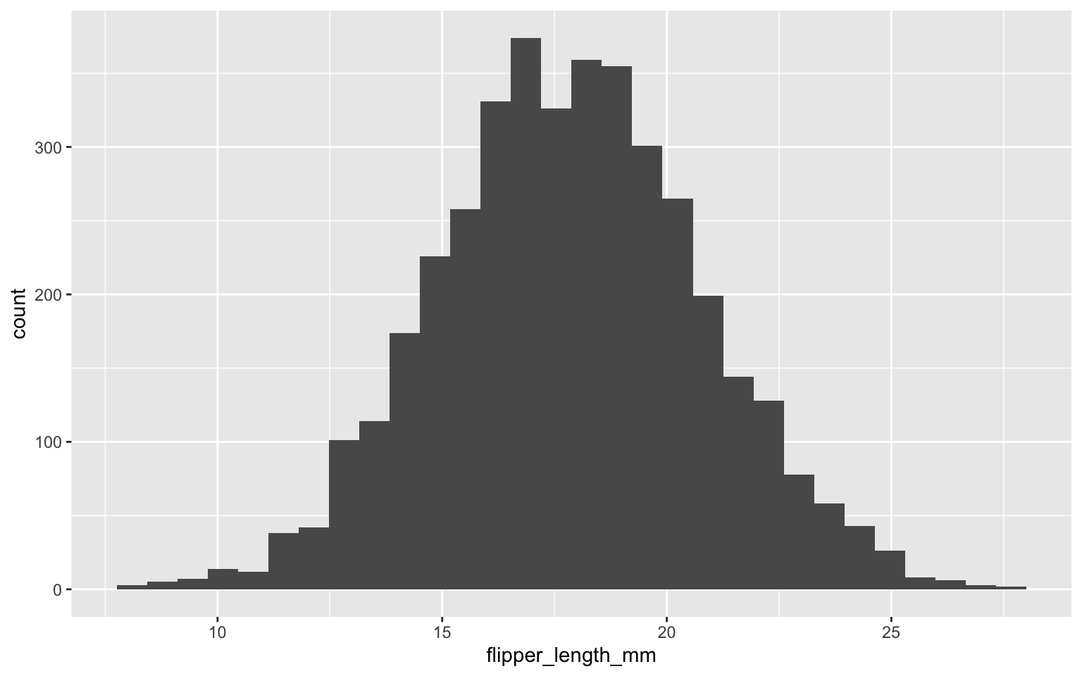
summary(echantillons$flipper_length_mm)
   Min. 1st Qu.  Median    Mean 3rd Qu.    Max.
  8.174  15.875  17.831  17.845  19.809  27.741
So, the algorithm converged around the value of 17.84 or 17.83 depending on whether we rely on the mean or the median of the samples. Visually, we can quickly see that describing the uncertainty around this parameter using the standard deviation will be perfectly appropriate, as the samples follow a nice normal curve.
We can also directly calculate all the probabilities that interest us, for example, the probability that the effect of wing length is greater than 20 g/mm:
sum(echantillons$flipper_length_mm>20)/length(echantillons$flipper_length_mm)
[1] 0.23125
However, the uncertainty is not necessarily symmetrical. For example, the one around the error parameter is rather asymmetrical:
echantillons |>
  ggplot(aes(sigma)) +
  geom_histogram()
`stat_bin()` using `bins = 30`. Pick better value with `binwidth`.
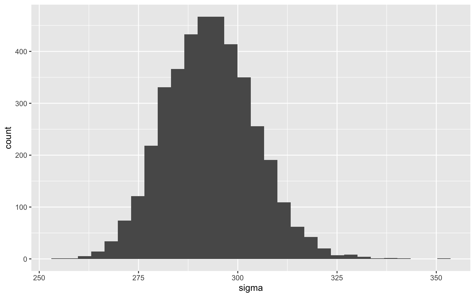
This is completely normal, if we think about the fact that the parameter is a variance term in the model and that variance can never be negative.
Since we have all the samples and we don’t take any shortcuts to estimate the uncertainty, we can directly evaluate this asymmetry:
quantile(echantillons$sigma, probs = c(0.015,.5,.985))
    1.5%      50%    98.5%
270.1696 292.7012 317.9939
The median of the parameter is about 293, but the bounds of the 97% credibility interval are 24 lower and 26 higher than the median.
As you can see, since you are breaking away from the arbitrary framework of the hypothesis testing approach, you can also drop the arbitrary value of 95% for confidence intervals, which has no theoretical basis or benefits. Your intervals are just as valid if they are 88% or 92% intervals.
This brings us to a major philosophical difference. Unlike the frequentist approach, the Bayesian approach does not have to comment on the distribution of residuals or their homogeneity before interpreting a model’s parameters. The parameters are what they are, and we can always interpret them as such (provided the MCMC process has run correctly, we will come back to this).
Beware, however, not to take shortcuts either. We do NOT know if wing length really affects penguin weight linearly at a rate of 17.8 mm/g. No model allows us to know that. What we do know is that IF we fit a linear model to do so, we measure a median increase of 17.8 mm/g.
And that’s the whole nuance. It is still important to observe the model’s residuals to see if it is well-suited to the data, if it is appropriate for the form of the relationships, etc. But deviations at this stage do not make the model uninterpretable. They are rather an indication that the model could be improved. A step in the iterative process.
Integrating prior information
We have so far avoided the subject, but we will not be able to continue for long without talking about it. One of the major contributions of the Bayesian approach is that it allows the integration of prior information into the calculation, before starting data collection. It is directly designed as a process of updating knowledge, rather than considering each experiment as independent.
The probability distribution associated with a parameter that we saw above is in fact the posterior probability. The updated version, after confronting our prior knowledge with the new data collected. It is here that, in general, tutorials on the Bayesian approach present Bayes’ theorem and its application, for example, to medical tests or doping, taking into account false positives, the baseline rate in the population, etc. All this is very interesting, but absolutely not necessary to get started with this approach.
The important thing is to understand, I repeat, that the results obtained are an update of prior knowledge by the data collected.
But what prior information should we use? There are several schools of thought on this.
Non-informative priors
One of the most reassuring things when starting with this approach is to know that it is possible to use priors so vague that they have no impact on the result. With this philosophy, our results are (in simple cases) identical to those found by the maximum likelihood approach (e.g., the glm or nlme function in R), with the difference that
- they can be interpreted within a Bayesian framework and
- we have access to all the samples of the posterior distribution to observe the distribution of the parameters, their correlations, etc.
In stan_glm, we could have applied non-informative priors, for example, by mentioning that for all we know, the parameters could be ABSOLUTELY ANYTHING. They could range from -Inf to +Inf with equal probabilities for each of the values.
m_noninformatif <- stan_glm(
  body_mass_g ~
    flipper_length_mm + bill_length_mm + sex + species,
  data = manchots,
  prior = NULL,
  prior_intercept = NULL,
  prior_aux = NULL
)
summary(m_noninformatif)
Model Info:
 function:     stan_glm
 family:       gaussian [identity]
 formula:      body_mass_g ~ flipper_length_mm + bill_length_mm + sex + species
 algorithm:    sampling
 sample:       4000 (posterior sample size)
 priors:       see help('prior_summary')
 observations: 333
 predictors:   6

Estimates:
                    mean    sd      10%     50%     90%
(Intercept)        -776.7   547.0 -1475.6  -778.7   -79.3
flipper_length_mm    17.9     2.9    14.2    18.0    21.6
bill_length_mm       21.8     7.2    12.6    21.8    31.0
sexmale             464.4    43.8   407.2   465.3   519.7
speciesChinstrap   -294.1    82.4  -398.5  -295.4  -186.1
speciesGentoo       704.0    95.4   579.0   704.7   827.2
sigma               293.2    11.5   278.7   292.8   307.9

Fit Diagnostics:
           mean   sd     10%    50%    90%
mean_PPD 4207.1   22.9 4178.2 4207.2 4236.5

The mean_ppd is the sample average posterior predictive distribution of the outcome variable (for details see help('summary.stanreg')).

MCMC diagnostics
                  mcse Rhat n_eff
(Intercept)       12.5  1.0 1930
flipper_length_mm  0.1  1.0 2276
bill_length_mm     0.2  1.0 2126
sexmale            0.9  1.0 2270
speciesChinstrap   1.8  1.0 2080
speciesGentoo      2.3  1.0 1769
sigma              0.2  1.0 3267
mean_PPD           0.4  1.0 3760
log-posterior      0.0  1.0 1566

For each parameter, mcse is Monte Carlo standard error, n_eff is a crude measure of effective sample size, and Rhat is the potential scale reduction factor on split chains (at convergence Rhat=1).
As expected, these results are almost identical to those obtained by the frequentist approach. AND also very close to those obtained with the default values, which we will discuss below.
Informative priors
At the other end of the prior spectrum, we might want to precisely integrate our knowledge of the subject before starting the experiment.
To simplify this section, we will work on a simple regression with a single parameter. The syntax for modifying the prior of a single parameter while keeping the other default values is not very user-friendly in stan_glm.
If, for example, an exploratory study on 20 penguins had found that the effect of wing length was 25 g/mm with a standard error of 10 g/mm, we could have integrated this information like this:
m_informatif_20 <- stan_glm(
  body_mass_g ~ flipper_length_mm,
  data = manchots,
  prior = normal(location = 25,scale = 10)
)
We will now compare this model to one where we use a non-informative prior on this slope:
m_informatif_0 <- stan_glm(
  body_mass_g ~ flipper_length_mm,
  data = manchots,
  prior = NULL
)
And one where we have a lot of certainty before starting the project. For example, we could have measured 10,000 penguins and found a mean of 25, but with a standard error of +/- 1 g/mm.
m_informatif_10000 <- stan_glm(
  body_mass_g ~ flipper_length_mm,
  data = manchots,
  prior = normal(location = 25,scale = 1)
)
summary(m_informatif_0)
Model Info:
 function:     stan_glm
 family:       gaussian [identity]
 formula:      body_mass_g ~ flipper_length_mm
 algorithm:    sampling
 sample:       4000 (posterior sample size)
 priors:       see help('prior_summary')
 observations: 333
 predictors:   2

Estimates:
                    mean    sd      10%     50%     90%
(Intercept)       -5873.6   314.8 -6279.8 -5874.8 -5478.8
flipper_length_mm    50.2     1.6    48.2    50.2    52.2
sigma               394.2    15.7   374.4   393.9   414.7

Fit Diagnostics:
           mean   sd     10%    50%    90%
mean_PPD 4207.5   30.2 4168.6 4207.0 4246.7

The mean_ppd is the sample average posterior predictive distribution of the outcome variable (for details see help('summary.stanreg')).

MCMC diagnostics
                  mcse Rhat n_eff
(Intercept)       5.2  1.0  3624
flipper_length_mm 0.0  1.0  3670
sigma             0.3  1.0  3729
mean_PPD          0.5  1.0  3463
log-posterior     0.0  1.0  1778

For each parameter, mcse is Monte Carlo standard error, n_eff is a crude measure of effective sample size, and Rhat is the potential scale reduction factor on split chains (at convergence Rhat=1).
summary(m_informatif_20)
Model Info:
 function:     stan_glm
 family:       gaussian [identity]
 formula:      body_mass_g ~ flipper_length_mm
 algorithm:    sampling
 sample:       4000 (posterior sample size)
 priors:       see help('prior_summary')
 observations: 333
 predictors:   2

Estimates:
                    mean    sd      10%     50%     90%
(Intercept)       -5747.9   306.1 -6132.3 -5749.7 -5358.2
flipper_length_mm    49.5     1.5    47.6    49.6    51.4
sigma               394.3    15.7   374.7   394.0   414.6

Fit Diagnostics:
           mean   sd     10%    50%    90%
mean_PPD 4208.1   30.9 4168.5 4207.9 4248.0

The mean_ppd is the sample average posterior predictive distribution of the outcome variable (for details see help('summary.stanreg')).

MCMC diagnostics
                  mcse Rhat n_eff
(Intercept)       5.1  1.0  3639
flipper_length_mm 0.0  1.0  3650
sigma             0.3  1.0  3745
mean_PPD          0.5  1.0  3935
log-posterior     0.0  1.0  1976

For each parameter, mcse is Monte Carlo standard error, n_eff is a crude measure of effective sample size, and Rhat is the potential scale reduction factor on split chains (at convergence Rhat=1).
summary(m_informatif_10000)
Model Info:
 function:     stan_glm
 family:       gaussian [identity]
 formula:      body_mass_g ~ flipper_length_mm
 algorithm:    sampling
 sample:       4000 (posterior sample size)
 priors:       see help('prior_summary')
 observations: 333
 predictors:   2

Estimates:
                    mean    sd      10%     50%     90%
(Intercept)       -1929.6   193.6 -2181.3 -1929.1 -1677.6
flipper_length_mm    30.5     1.0    29.3    30.5    31.8
sigma               480.8    20.0   455.5   480.1   507.0

Fit Diagnostics:
           mean   sd     10%    50%    90%
mean_PPD 4206.8   36.6 4159.3 4207.2 4253.2

The mean_ppd is the sample average posterior predictive distribution of the outcome variable (for details see help('summary.stanreg')).

MCMC diagnostics
                  mcse Rhat n_eff
(Intercept)       3.5  1.0  3051
flipper_length_mm 0.0  1.0  3052
sigma             0.3  1.0  3311
mean_PPD          0.6  1.0  3476
log-posterior     0.0  1.0  1990

For each parameter, mcse is Monte Carlo standard error, n_eff is a crude measure of effective sample size, and Rhat is the potential scale reduction factor on split chains (at convergence Rhat=1).
We therefore find that there is very little difference between the model with a very vague prior and the one based on a preliminary study. In both cases, the new data provide a lot of information compared to our prior knowledge. On the other hand, in the third model, which uses a solid study with 10,000 individuals as a prior, the posterior distribution of the parameter is at 30 g/mm (vs. 50 g/mm for the other two), because in this case, our prior knowledge was very strong. Even if our study on hundreds of penguins finds a higher value, our knowledge about penguins changes little.
This is the full power of the Bayesian approach. It encapsulates our process of updating knowledge. If we have little or no information about the phenomenon before starting, the analysis lets the data speak. But if our knowledge was solid, it will be difficult to shake.
I always like to think of the Bayesian approach with informative priors as a permanent meta-analysis. Each study moves the synthesis of our knowledge. Proportionately to the amount of information known before and provided by the new data.
Weakly informative priors
Although at first glance non-informative priors are attractive due to their appearance of objectivity, they are rarely the most appropriate.
First of all, from a technical point of view, they make the task of our MCMC very complex, since the latter must explore essentially from -Inf to +Inf for each of the parameters. Also, they are not very realistic, since we know that it is not as likely to have a slope of 0 g/mm as one of 50 g/mm or one of 5,000,000 g/mm. Just by the range of weight and wing length of a penguin, we know that this is not possible.
There is therefore a compromise, which is becoming increasingly popular, for cases where we do not have precise information like a preliminary study, but still have an idea of the order of magnitude of the possibilities: weakly informative priors. To facilitate their understanding, these are often based on standardized data (i.e., centered and scaled) and are therefore expressed in terms of standard deviation.
This is the strategy used by stan_glm. Unless otherwise specified (as above), the latter places a weak prior on your slopes, based on a normal distribution, with a mean of 0 and a standard deviation of 2.5, after having standardized your data. So, before starting the fit, the model assumes that there is a 95% chance that the slope (on the standardized scale) will be between -5 and +5 standard deviations of Y for one standard deviation of X. This seemingly “ordinary” number is in fact extremely high.
For example, the standardized effect size of Cohen’s D, which is precisely in standard deviations of Y for a change of one standard deviation of X, is interpreted as a small effect around 0.1, a large effect around 0.8, and a huge effect around 2. This strategy therefore constrains the parameters within reasonable value ranges, while leaving ample freedom for the data to express themselves.
Since the normal distribution extends from -Inf to +Inf, if you ever find a crazy relationship with a standardized slope of 10 or 50 standard deviations, the model will still be able to fit it, as long as you have the data to support it. Otherwise, the model will remain skeptical, as you should too.
To what extent do new data change our knowledge?
One of the most direct ways to see if the collected data are meaningful or not is to compare the prior distribution and the posterior distribution of our parameters side by side. In rstanarm, the posterior_vs_prior function automates this task.
For example, let’s compare the evolution of the parameter for the effect of wing length, between our model with a little information (n=20) and our model with a lot of information (n=10000):
posterior_vs_prior(m_informatif_20,"flipper_length_mm")
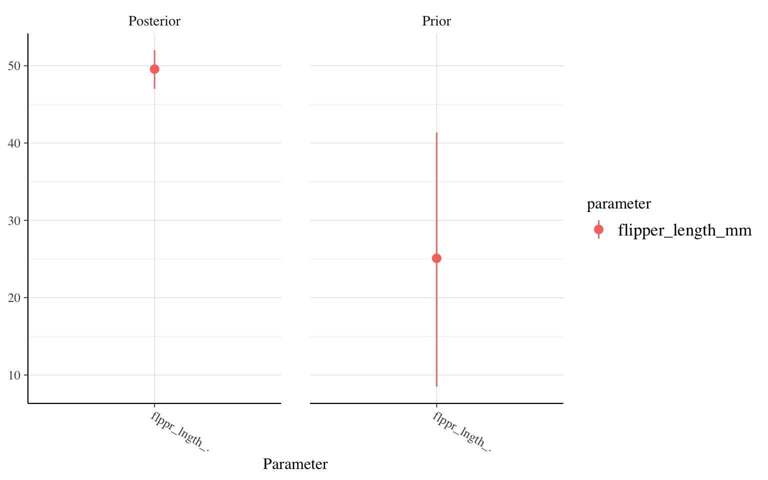
posterior_vs_prior(m_informatif_10000,"flipper_length_mm")
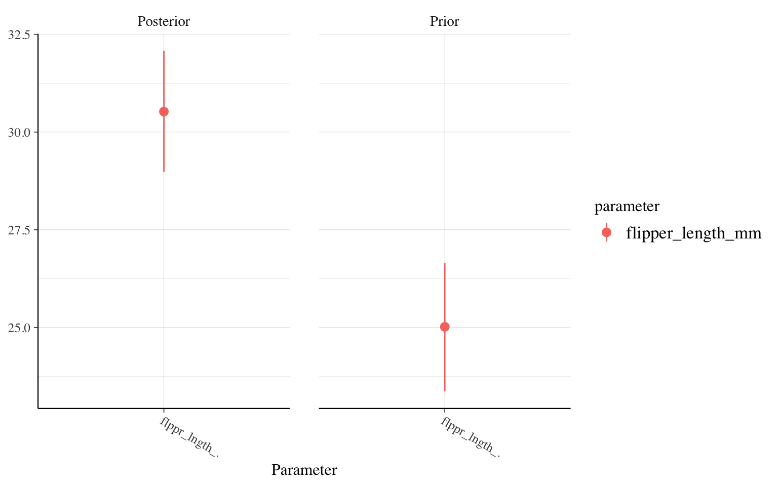
The lesson of prior distributions
The thing to remember from this discussion about prior distributions is therefore that they are a way of being transparent about your assumptions. To define what you know about the phenomenon before you start. It is not a way to “cheat” or manipulate the results. The Bayesian process of parameter estimation is designed specifically to update knowledge based on new data. It is made to let your data speak for themselves.
Do my priors make sense?
One important thing to ask yourself when applying prior distributions to our models is: do these distributions make sense for understanding the phenomenon under study? We are not talking here about using the project data to calculate prior distributions in advance, that would be very dangerous: a serious form of overfitting.
However, we must absolutely take a look at the relationships that are implicit in our priors. We must ask ourselves: is it realistic or not that we would observe such relationships? The more complex your models become, the more it can become impossible to mentally manage this type of question. This is why it is usually recommended to perform a prior predictive check. The principle of this technique is to sample data, not from the posterior distribution, but directly from the prior distribution.
In rstanarm, we can achieve this directly by fitting our model with an additional argument:
a_priori_10000 <- stan_glm(
  body_mass_g ~ flipper_length_mm,
  data = manchots,
  prior = normal(location = 25,scale = 1),
  prior_PD = TRUE
)
We can then look, for example, at the distribution of expected weight values:
pp_check(a_priori_10000)
Obviously, this is not perfect. We find some weight distributions with values < 0 and some centered on weights 2x greater than the originals. But these instances are very rare. The majority of the distributions would have made sense ecologically.
We could also extract and plot each of the slopes (or here a sample of 100 so that it remains readable). The a_priori_10000 object already contains a series of parameter samples, which we can extract using the as.data.frame() function.
verif_pentes <- a_priori_10000 |>
  as.data.frame() |>
  janitor::clean_names() |>
  sample_n(100)
head(verif_pentes)
   intercept flipper_length_mm      sigma
1 -2872.7168          24.82238  251.56464
2 -2065.1517          23.82648 1649.60026
3 -3229.8383          25.38553  485.41520
4  -907.2649          25.12735  366.63444
5 -2161.4786          25.30185  626.57642
6 -1154.2419          22.77948   27.41661
verif_pentes |>
  ggplot() +
  geom_abline(aes(
    slope = flipper_length_mm,
    intercept = intercept)) +
  xlim(170,240) +
  ylim(2500,7000)
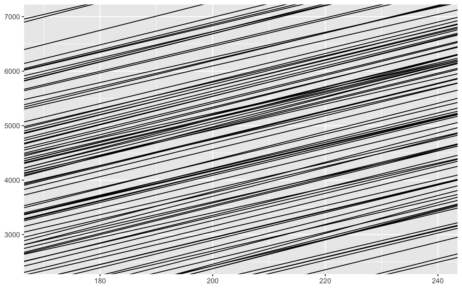
Note that the geom_abline layer does not build the graph limits. We had to do it manually.
Here, the slopes are very tight around values that make a lot of sense, since it was our model with a very strong prior.
Let’s now compare with the default weakly informative priors in rstanarm.
stan_glm(
  body_mass_g ~ flipper_length_mm,
  data = manchots,
  prior_PD = TRUE
) |>
  as.data.frame() |>
  janitor::clean_names() |>
  sample_n(100) |>
  ggplot() +
  geom_abline(aes(
    slope = flipper_length_mm,
    intercept = intercept)) +
  xlim(170,240) +
  ylim(2500,7000)
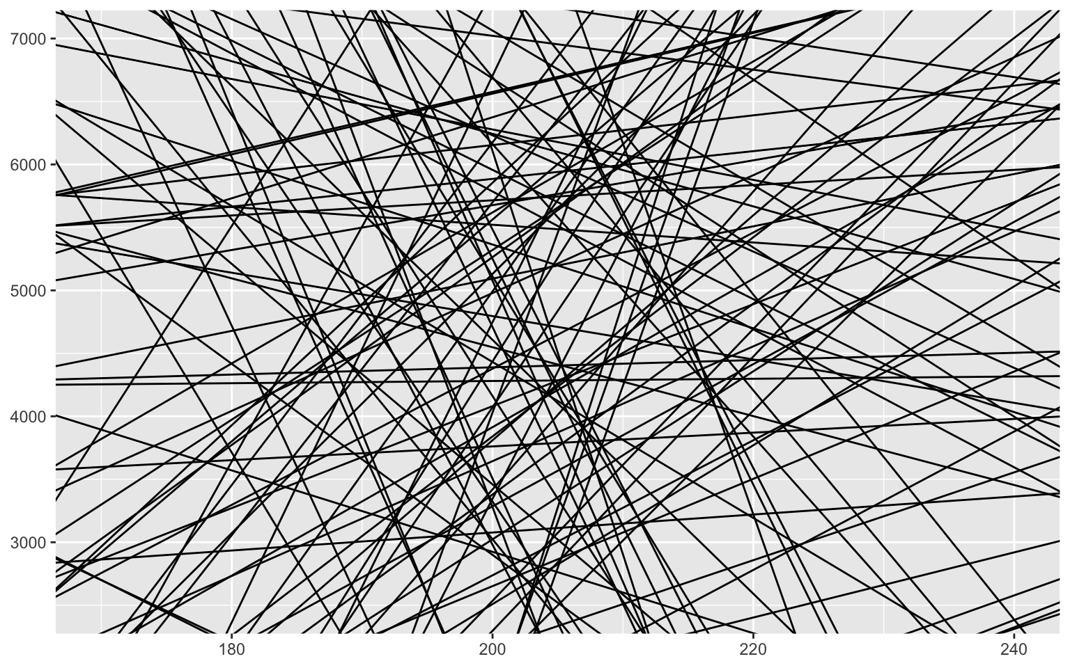
You can see that the default prior does not force anything on our model. A slope is as likely to be positive as it is to be negative, and most are rather weak, close to a slope of zero. Some predict extremely large weights (we can guess several > 10,000g), but in general, the majority is very good. This is what we want to find.
Did my MCMC work well?
So far, we have used and explained MCMCs very briefly, but it is important to know that they do not magically always arrive at the right result.
THE thing to check is whether each of the chains mixed well. That is, did it properly explore the landscape around each parameter and not get stuck in a small area?
Visual check
We can first check the mixing of the chains visually, using, for example, the mcmc_trace function from the bayesplot library:
library(bayesplot)
mcmc_trace(m_informatif_0)
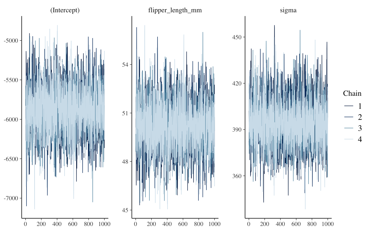
The function therefore displays the posterior distribution sampling process, with one panel per parameter. Here, we have 4 chains, since if we don’t mention anything, this is the number of chains that rstanarm launches in parallel. The advantage of using multiple chains is that we can see if they behaved in an equivalent way, among themselves and throughout the process. What we want to see, for each, is a kind of fuzzy caterpillar across the entire width of the panel. What would be worrying to find would be, for example, that one of the chains is only half the height of the others, or that it starts with very large values for a few hundred iterations, etc.
R-hat?
Since it can sometimes be difficult to visually interpret these graphs, a measure, named R-hat, was invented to guide us. Simply put, it is calculated as the square root of the ratio between the total variance of the samples and the average intra-chain variance. If R-hat is close to 1, the chains are well mixed and we can trust the result. If the value moves away from 1 (the threshold of 1.01 is often cited), then the chains are not well mixed. The posterior distribution has not been well explored and the result is not usable. Moreover, rstanarm will display a warning if this is the case.
These values are accessible in several places, for example, at the end of our model’s summary:
summary(m_informatif_0)
Model Info:
 function:     stan_glm
 family:       gaussian [identity]
 formula:      body_mass_g ~ flipper_length_mm
 algorithm:    sampling
 sample:       4000 (posterior sample size)
 priors:       see help('prior_summary')
 observations: 333
 predictors:   2

Estimates:
                    mean    sd      10%     50%     90%
(Intercept)       -5873.6   314.8 -6279.8 -5874.8 -5478.8
flipper_length_mm    50.2     1.6    48.2    50.2    52.2
sigma               394.2    15.7   374.4   393.9   414.7

Fit Diagnostics:
           mean   sd     10%    50%    90%
mean_PPD 4207.5   30.2 4168.6 4207.0 4246.7

The mean_ppd is the sample average posterior predictive distribution of the outcome variable (for details see help('summary.stanreg')).

MCMC diagnostics
                  mcse Rhat n_eff
(Intercept)       5.2  1.0  3624
flipper_length_mm 0.0  1.0  3670
sigma             0.3  1.0  3729
mean_PPD          0.5  1.0  3463
log-posterior     0.0  1.0  1778

For each parameter, mcse is Monte Carlo standard error, n_eff is a crude measure of effective sample size, and Rhat is the potential scale reduction factor on split chains (at convergence Rhat=1).
You can see that all Rhat values are rounded to 1.0.
Effective sample size
You also notice another diagnostic tool in this output: n_eff. n_eff measures the number of effective samples that your chains have produced, taking into account the temporal autocorrelation present in the chains. If this number is particularly low, it is a sign that you have re-sampled the same area of the posterior distribution many times, and that your conclusions are probably not representative of its true form. You will often read that you must obtain at least 1000 effective samples to have a usable portrait.
Solution to problems with the MCMC process
The simplest thing to do when you encounter problems with your chains is simply to ask them to sample more.
For example, we could ask to explore 2000 samples per chain instead of 1000, like this:
m2000 <- stan_glm(
  body_mass_g ~ flipper_length_mm,
  data = manchots,
  prior = NULL,
  iter = 4000
)
summary(m2000)
Model Info:
 function:     stan_glm
 family:       gaussian [identity]
 formula:      body_mass_g ~ flipper_length_mm
 algorithm:    sampling
 sample:       8000 (posterior sample size)
 priors:       see help('prior_summary')
 observations: 333
 predictors:   2

Estimates:
                    mean    sd      10%     50%     90%
(Intercept)       -5867.1   307.6 -6252.6 -5871.9 -5476.6
flipper_length_mm    50.1     1.5    48.2    50.2    52.0
sigma               394.8    15.4   375.6   394.2   414.9

Fit Diagnostics:
           mean   sd     10%    50%    90%
mean_PPD 4206.3   30.7 4166.7 4206.6 4245.2

The mean_ppd is the sample average posterior predictive distribution of the outcome variable (for details see help('summary.stanreg')).

MCMC diagnostics
                  mcse Rhat n_eff
(Intercept)       3.6  1.0  7468
flipper_length_mm 0.0  1.0  7499
sigma             0.2  1.0  8193
mean_PPD          0.4  1.0  7325
log-posterior     0.0  1.0  3911

For each parameter, mcse is Monte Carlo standard error, n_eff is a crude measure of effective sample size, and Rhat is the potential scale reduction factor on split chains (at convergence Rhat=1).
Note that to get 2000 samples per chain, I had to request 4000 in total, because, unless otherwise specified, rstanarm instructs the algorithm to use half of the iterations to evaluate the chain’s meta-parameters (e.g., how big to make the jumps between proposals, etc.), which it calls the warm-up. If necessary (for example, if a warning suggests it), you can also change the number of iterations allocated to the warm-up.
That being said, most of the time, if you’re having trouble with your chains, it’s more likely that your model is misspecified. Do your priors make sense in relation to the data? Do you have, for example, an observation worth 1,000,000, while your prior is specified as N(0,3), and therefore, it is almost impossible to obtain such large values?
Hence the importance of properly performing the prior predictive check.
Is my model good?
Without hypothesis testing, you may feel a little lost when it comes to evaluating the quality of your statistical model!
As mentioned above, the first thing to remember is that if your chains have correctly sampled the posterior distribution, your model IS interpretable. Your parameters answer the question: assuming this model and the measured data, here are the most probable values for each of the model’s parameters. So, the question here is not to test the model as such, but to explore it.
One of the first tools at your disposal is to see if the distribution of predictions, based on the posterior distribution of the parameters, adequately reconstructs the original distribution of the explained variable. This technique is called a posterior predictive check.
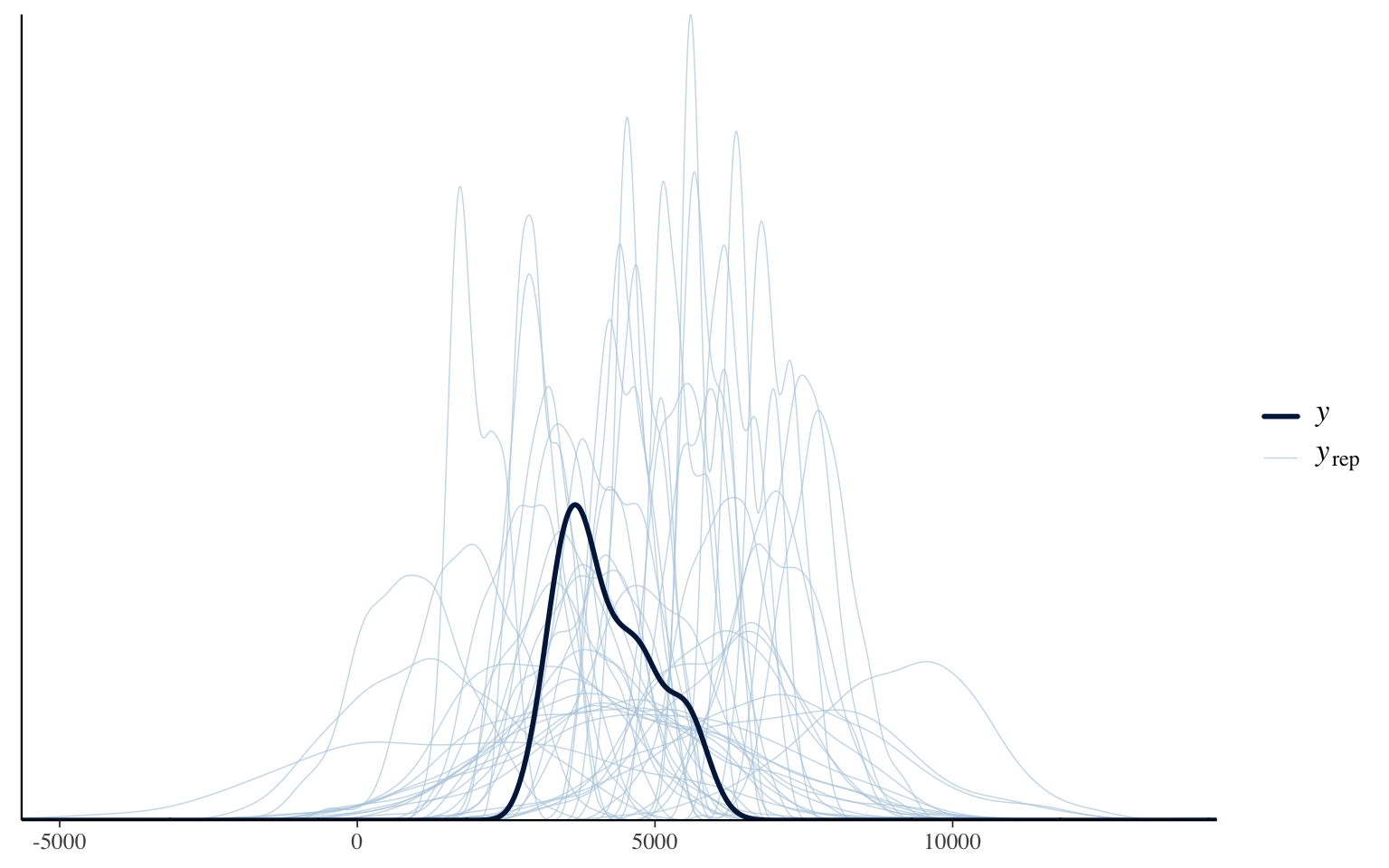
pp_check(m_informatif_0)
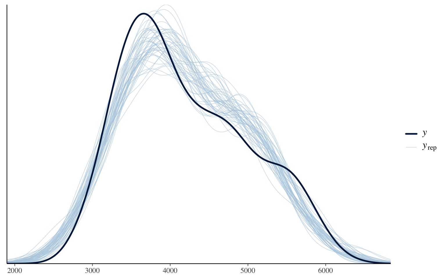
This graph compares the original (smoothed) data distribution (the black line) with the distribution of predictions for each of the parameter combinations tested by the model. In general, our model adequately manages to reproduce the original distribution. I remind you, again here, it is not a test, but an exploration. If ever particularities of the data are not well reproduced or the general shape is not respected, it is a sign that a better model can probably be designed for these data.
Is this model better than another?
After exploring the fit of your model, you will probably want to know if it is an improvement over other models you have tested. Are you moving in the right direction or not?
To do this, we will have to agree on a way to measure the quality of the model. One of the dilemmas you may be aware of regarding the quality of statistical models is that they can end up being overfitted to the data found. With enough parameters, you can reproduce any data set with precision, even perfection. But this perfect model would be of no use because it would be completely useless when faced with new data. The adage also says: fitting is easy, predicting is hard. However, what we want is a model that can predict correctly. That’s the only way it becomes useful.
This is why the recommended way to evaluate the quality of a statistical model is to use cross-validation. In its most extreme version, this strategy consists of fitting the model with all the data except one. Then, we evaluate the quality of the prediction for the data left aside. Then we repeat the process with each of the data points! This particular version is usually called leave-one-out cross validation (loo-cv).
With simple models that are quick to fit, it can be relatively easy to code cross-validation in a loop and run it in a few seconds. In real life, however, this way of doing things is rarely practical. Even if your model is relatively quick to fit, for example, 30 seconds per fit, this operation could still take tens of hours if you have a few thousand observations, which is not uncommon.
WAIC
You may not know this, but the AIC (Akaike Information Criterion) was designed precisely as an approximation, a shortcut, to obtain the information from a cross-validation, without the computational burden it implies. At large sample sizes, AIC and loo-cv will provide exactly the same ranking for a series of models.
There is, for the Bayesian approach, a similar algorithm to AIC, the WAIC, which correctly takes into account the fact that our Bayesian model provides us with a series of parameter values rather than a direct value. The latter can be used in the same way as AIC, with delta-AIC, Akaike weights allowing us to determine the probability that each model is the best, etc.
However, it is not currently the recommended metric to compare models with each other, because another algorithm, PSIS-LOO-CV, can almost always do a more precise job, in addition to directly informing the user when its values become imprecise/dangerous to use.
PSIS-LOO-CV
As with AIC, PSIS-LOO-CV is an algorithm that makes it possible to obtain the results of cross-validation on a model without having to refit it for each of the predictions.
The general idea is that it is possible for each observation and for each parameter sample to measure the probability of observing this value. The inverse of this probability will therefore be the weight of its contribution to the model. The more surprising an observation is, the more influence it will have had. Then, rather than considering each parameter sample as equal in the mean calculations, we weight them by the weight of each observation. This technique is called importance sampling.
One of the problems with this strategy is that the weights are not necessarily reliable. If they are particularly large, they can dominate the calculation. We could obviously cut the weights beyond a threshold, but that too would create a bias in the calculation. The key to solving this problem is that, according to the theory, the large weight values should follow a Pareto distribution for each observation. The PSIS-LOO-CV algorithm (Pareto-Smoothed Importance Sampling) therefore replaces the large weights with the smoothed values, predicted by the Pareto distribution for that observation.
The main advantage of this method over WAIC is that it provides for each observation the parameter k of the Pareto distribution that was estimated, and that this can be used to
- Identify influential values (large k values)
- Identify the moments when the PSIS-LOO-CV value is not reliable. The tail of the Pareto distribution becomes extremely wide beyond k > 0.5, and therefore the associated estimates are less reliable. Simulations suggest that PSIS-LOO-CV values are no longer usable beyond k > 0.7, and you will get warnings when the time comes.
However, like AIC, the PSIS-LOO-CV value of a single model is absolutely not informative and cannot be interpreted as the quality of the model as such. It is a relative measure of quality.
Usage example
To see how to apply model comparison with PSIS-LOO-CV, we will compare the model from the beginning of the workshop that had 4 variables to the one used for the priors, which contained only one.
loo(m_bayes)
Computed from 4000 by 333 log-likelihood matrix.

         Estimate   SE
elpd_loo  -2366.7 12.3
p_loo         6.6  0.5
looic      4733.3 24.7
------
MCSE of elpd_loo is 0.0.
MCSE and ESS estimates assume MCMC draws (r_eff in [0.5, 1.2]).

All Pareto k estimates are good (k < 0.7).
See help('pareto-k-diagnostic') for details.
loo(m_informatif_20)
Computed from 4000 by 333 log-likelihood matrix.

         Estimate   SE
elpd_loo  -2464.1 13.1
p_loo         2.9  0.3
looic      4928.3 26.2
------
MCSE of elpd_loo is 0.0.
MCSE and ESS estimates assume MCMC draws (r_eff in [0.8, 1.0]).

All Pareto k estimates are good (k < 0.7).
See help('pareto-k-diagnostic') for details.
So, the first thing to know: PSIS-LOO-CV measures the precision of the predictions. Therefore, the higher the value, the better the model. Here, the m_bayes model, which contains 4 variables, produces better predictions than the one with only one variable. Its elpd_loo value (another name for PSIS-LOO-CV) is -2464.1 vs. -2366.7.
Since we have all the samples, the algorithm was also able to calculate the variability around our PSIS-LOO-CV estimate, which is 13.1 on one side and 12.3 on the other.
We can therefore ask what the real difference is between these models. We could go and retrieve the numbers for each of the parameter samples ourselves, but the loo_compare function will do it for us automatically:
loo_compare(loo(m_bayes), loo(m_informatif_20))
                elpd_diff se_diff
m_bayes           0.0       0.0
m_informatif_20 -97.5      11.6
So, the average PSIS-LOO-CV difference between our two models is -97.5 points, with a standard error of 11.6 points. The difference is really clear between the two models.
Conclusion
And that’s it. It’s no more complicated than that to make the transition to Bayesian analysis in 2025.
You now have the basics to:
-
Fit your models in a Bayesian framework (
stan_glmfrom therstanarmlibrary) with weakly informative priors. -
The ability to integrate non-informative or informative priors as you wish.
-
The tools to explore your Markov chains to ensure that they have properly explored the posterior distribution of the parameters (visual check, Rhat, n_eff).
-
Compare your models in a Bayesian framework, again using all the information from the posterior distribution with PSIS-LOO-CV.
We have, of course, only scratched the surface of the potential of this approach. For what comes next, several paths are open to you:
-
Explore the other functions of the
rstanarmlibrary, which reproduce the functionalities oflmer,nlme, etc. -
Use the
brmslibrary and itsbrmfunction to create your models. Whilerstanarmwas designed from a more educational perspective,brmswas designed as a general tool, in which you can fit just about any model that a graduate student might need in environmental sciences. In addition,brmshas astancodefunction, which allows you to inspect the Stan code that was generated for you, to quietly start looking under the hood. -
Read the book Statistical Rethinking by Richard McElreath. This book is usually recommended as THE book to get started with Bayesian approaches without getting bogged down in mathematical details. McElearth is an excellent storyteller and the book is surprisingly entertaining.
-
Read the book Regression and Other Stories by Gelman, Hill & Vehtari. This book essentially reviews the introductory statistics curriculum, but in a Bayesian framework (without too much emphasis), using the functions of the
rstanarmlibrary and a very practical rather than theoretical approach. This book is also highly recommended.