Big Data Manipulation
Roxanne Giguère-Tremblay & Arthur de Grandpré
May 2021
- Context : Big Data
- The data.table package
- Packages
- Data
- The vroom package
- References
Context : Big Data
What is “Big Data”? Databases that are considered big data are so large that normal database management tools have great difficulty in performing the manipulations required and their handling time becomes excessively long and non-productive.
Where do we find big data in Environmental Sciences? - GIS - Global monitoring - climate change - Climate modelling - Microbial ecology with genomics - Citizen participation via applications such as Ebird (for example) - etc…
What are the benefits of Big Data? First, at the statistical level, having a lot of data helps to compensate for the possibility that some data greatly influences the results via the sample size effect. That is, when we have a little set of data, an outlier point will probably influence the outcome of our analysis. However, if this same outlier point ends up in a very big data set, it will have less impact on the final result.
Second, at a more global level, Big Data allows for better environmental monitoring and fairer decisions about environmental laws as analyses and models are fairer and more reliable than before.
In this workshop… For these reasons and because many of us are probably already using Big Data in our research, it seems relevant to offer this workshop. The latter will allow us to be more efficient and above all faster in handling our data.
Although the word “Big Data” can be scary, it is possible to manipulate them without too many complexities and that is what we will see today. We’ll see the basic outlines of what can be done with R data.table and Vroom packages. Several references are also available if you want to learn more about the packages or if you have questions that are not presented in the workshop.
The data.table package
Introduction
Let’s start with the data.table package. This R package is used for data manipulation in table form, as is the default function of data.frame. However, it is much faster and for some people it also has a more intuitive syntax than the default function. Another advantage is that a database in the form of a data.table can be used in the same way as a data.frame in different packages such as ggplot2, for example.
An important piece of information to know about this package is that it has won each of the many comparison exercises that have been performed against dplyr and even with panda in Python. Thus, it is one of the important packages to know in Data Science.
Noted that the tutorial I am presenting today is greatly inspired from this one: https://www.machinelearningplus.com/data-manipulation/datatable-in-r-complete-guide/.
Installation
Packages
The data.table package can be installed using either CRAN for the latest stable build, or Github for the newest features.
# installing data.table
# from CRAN
install.packages('data.table')

# from Github
install.packages("data.table",
                 repos="https://Rdatatable.gitlab.io/data.table")

# check version and update
data.table::update.dev.pkg() # Workshop built on version 1.14.1.

# load the library
library("data.table")
Data
Set the directory
#setwd("C:/Users/Arthur/Desktop/bigdata_web") # Change for your own directory!
In this course we will use the data set abalone in the AppliedPredictiveModeling package.
# Installation du package AppliedPredictiveModeling pour télécharger le dataset qui sera utilisé pour l'atelier
install.packages("AppliedPredictiveModeling")
You can download it here and save it on your R project directly on your computer.
library("AppliedPredictiveModeling")

 data("abalone")
 dset <- abalone
 head(dset)

##   Type LongestShell Diameter Height WholeWeight ShuckedWeight VisceraWeight
## 1    M        0.455    0.365  0.095      0.5140        0.2245        0.1010
## 2    M        0.350    0.265  0.090      0.2255        0.0995        0.0485
## 3    F        0.530    0.420  0.135      0.6770        0.2565        0.1415
## 4    M        0.440    0.365  0.125      0.5160        0.2155        0.1140
## 5    I        0.330    0.255  0.080      0.2050        0.0895        0.0395
## 6    I        0.425    0.300  0.095      0.3515        0.1410        0.0775
##   ShellWeight Rings
## 1       0.150    15
## 2       0.070     7
## 3       0.210     9
## 4       0.155    10
## 5       0.055     7
## 6       0.120     8

#
#.csv creation
 write.csv(dset, "abalone.csv")
Reading data
Even though data.frame and data.table objects are similar, they are not used in the same way; data.table uses a more intuitive syntax.
The fread function (fast read) is equivalent to read.csv. It can import local or remote csv files approximately 20 times faster than read.csv. It also generates a data.table format object.
Since objects of class data.table are made from a data.frame, all functions accepting a data.frame should work with data.table
dset <- fread("abalone.csv")
head(dset) # To visualy confirm data structure

##    V1 Type LongestShell Diameter Height WholeWeight ShuckedWeight VisceraWeight
## 1:  1    M        0.455    0.365  0.095      0.5140        0.2245        0.1010
## 2:  2    M        0.350    0.265  0.090      0.2255        0.0995        0.0485
## 3:  3    F        0.530    0.420  0.135      0.6770        0.2565        0.1415
## 4:  4    M        0.440    0.365  0.125      0.5160        0.2155        0.1140
## 5:  5    I        0.330    0.255  0.080      0.2050        0.0895        0.0395
## 6:  6    I        0.425    0.300  0.095      0.3515        0.1410        0.0775
##    ShellWeight Rings
## 1:       0.150    15
## 2:       0.070     7
## 3:       0.210     9
## 4:       0.155    10
## 5:       0.055     7
## 6:       0.120     8

class(dset) # To confirm object class

## [1] "data.table" "data.frame"
Even though fread reads data faster than read.csv, it doesn’t really show when reading small datasets. The difference becomes larger when using very large or complexe datasets (Big Data).
We will create a bigger data set (1M lines) that will allow us to visualize the read speed difference between read.csv and fread.
# Create a large .csv file
set.seed(100) # set random seed so all runs are the same
m <- data.frame(matrix(runif(1000000), nrow=1000000))
write.csv(m, "m2.csv", row.names = F)

# Time taken by read.csv to import
system.time({m_df <- read.csv("m2.csv")})

##    user  system elapsed
##   2.135   0.066   2.219

# Time taken by fread to import
system.time({m_dt <- fread("m2.csv")})

##    user  system elapsed
##   0.045   0.008   0.053
Converting a data.frame into a data.table
Conversion from data.frame to data.table can be done using two different functions :
- data.table() or as.data.table()
- setDT()
The main difference between both functions is that the first creates a copy while the second directly modifies the original object.
The first function as.data.table() does not include row names, so they must be reassigned if necessary.
1st function :
dset_dt <- as.data.table(dset) # Conversion vers DT
class(dset_dt) # Le data.table est fait à partir d'un data.frame

## [1] "data.table" "data.frame"

rownames(dset_dt) = rownames(dset)
dset_dt

##         V1 Type LongestShell Diameter Height WholeWeight ShuckedWeight
##    1:    1    M        0.455    0.365  0.095      0.5140        0.2245
##    2:    2    M        0.350    0.265  0.090      0.2255        0.0995
##    3:    3    F        0.530    0.420  0.135      0.6770        0.2565
##    4:    4    M        0.440    0.365  0.125      0.5160        0.2155
##    5:    5    I        0.330    0.255  0.080      0.2050        0.0895
##   ---
## 4173: 4173    F        0.565    0.450  0.165      0.8870        0.3700
## 4174: 4174    M        0.590    0.440  0.135      0.9660        0.4390
## 4175: 4175    M        0.600    0.475  0.205      1.1760        0.5255
## 4176: 4176    F        0.625    0.485  0.150      1.0945        0.5310
## 4177: 4177    M        0.710    0.555  0.195      1.9485        0.9455
##       VisceraWeight ShellWeight Rings
##    1:        0.1010      0.1500    15
##    2:        0.0485      0.0700     7
##    3:        0.1415      0.2100     9
##    4:        0.1140      0.1550    10
##    5:        0.0395      0.0550     7
##   ---
## 4173:        0.2390      0.2490    11
## 4174:        0.2145      0.2605    10
## 4175:        0.2875      0.3080     9
## 4176:        0.2610      0.2960    10
## 4177:        0.3765      0.4950    12
2nd function
dset_copy <- copy(dset)
setDT(dset_copy)
class(dset_copy)

## [1] "data.table" "data.frame"
Converting a data.table to data.frame
If you wish to convert a data.table into a data.frame, it is just as simple using the setDF() or as.data.frame() functions
setDF(dset_copy)
class(dset_copy)

## [1] "data.frame"
Data manipulations
Conditionnal filtering
One of the main differences between both types of datasets is that data.table knows the names of its columns. This makes code writing more intuitive.
This is and example of the syntax used to filter a data.frame :
head(dset_copy[dset_copy$Type == "M" & dset_copy$Rings == 10, ]) # lines where type is M with 10 rings

##      V1 Type LongestShell Diameter Height WholeWeight ShuckedWeight
## 4     4    M        0.440    0.365  0.125      0.5160        0.2155
## 12   12    M        0.430    0.350  0.110      0.4060        0.1675
## 31   31    M        0.580    0.470  0.165      0.9975        0.3935
## 53   53    M        0.485    0.360  0.130      0.5415        0.2595
## 88   88    M        0.560    0.440  0.160      0.8645        0.3305
## 104 104    M        0.530    0.415  0.140      0.7240        0.3105
##     VisceraWeight ShellWeight Rings
## 4          0.1140       0.155    10
## 12         0.0810       0.135    10
## 31         0.2420       0.330    10
## 53         0.0960       0.160    10
## 88         0.2075       0.260    10
## 104        0.1675       0.205    10
While the syntax for a data.table goes like this :
-
DT[i, j, by] where i = line filter, j = column selection, by = grouping
head(dset_dt[Type== “M” & Rings== 10, ]) # lines where type is M with 10 rings and no grouping
## V1 Type LongestShell Diameter Height WholeWeight ShuckedWeight ## 1: 4 M 0.440 0.365 0.125 0.5160 0.2155 ## 2: 12 M 0.430 0.350 0.110 0.4060 0.1675 ## 3: 31 M 0.580 0.470 0.165 0.9975 0.3935 ## 4: 53 M 0.485 0.360 0.130 0.5415 0.2595 ## 5: 88 M 0.560 0.440 0.160 0.8645 0.3305 ## 6: 104 M 0.530 0.415 0.140 0.7240 0.3105 ## VisceraWeight ShellWeight Rings ## 1: 0.1140 0.155 10 ## 2: 0.0810 0.135 10 ## 3: 0.2420 0.330 10 ## 4: 0.0960 0.160 10 ## 5: 0.2075 0.260 10 ## 6: 0.1675 0.205 10
Column selection
Selecting columns in one of the most frequent database manipulation. Unlike a data.frame, a data.table can be subseted using its column names instead of their indexes, without quotation marks to obtain a vector, and with quotation marks to obtain a table.
# for a vector
head(dset_dt[, Diameter])

## [1] 0.365 0.265 0.420 0.365 0.255 0.300

# for a table
head(dset_dt[, "Diameter"])

##    Diameter
## 1:    0.365
## 2:    0.265
## 3:    0.420
## 4:    0.365
## 5:    0.255
## 6:    0.300

# equivalent to
# dset_dt[, .(Diameter)]
# equivalent to
# dset_dt[, 3]
Selecting multiple columns
To select multiple columns, use a vector of the column names you want to select.
head(dset_dt[,.(Type, Diameter, Rings)])

##    Type Diameter Rings
## 1:    M    0.365    15
## 2:    M    0.265     7
## 3:    F    0.420     9
## 4:    M    0.365    10
## 5:    I    0.255     7
## 6:    I    0.300     8

# equivalent to
# dset_dt[,c("Type","Diameter","Rings")]
# equivalent to
# dset_dt[,c(1,3,9)]
Dropping columns
To drop columns from the dataset, use the ! negation operator before the vector of columns to exclude.
drop_cols <- c("Height", "ShuckedWeight")
head(dset_dt[, !drop_cols, with = FALSE]) # Setting with = FALSE disables the ability to refer to columns as if they are variables, thereby restoring the “data.frame mode”

##    V1 Type LongestShell Diameter WholeWeight VisceraWeight ShellWeight Rings
## 1:  1    M        0.455    0.365      0.5140        0.1010       0.150    15
## 2:  2    M        0.350    0.265      0.2255        0.0485       0.070     7
## 3:  3    F        0.530    0.420      0.6770        0.1415       0.210     9
## 4:  4    M        0.440    0.365      0.5160        0.1140       0.155    10
## 5:  5    I        0.330    0.255      0.2050        0.0395       0.055     7
## 6:  6    I        0.425    0.300      0.3515        0.0775       0.120     8

# equivalent to
# dset_dt[, !c("Height", "ShuckedWeight")]
# equivalent to
# dset_dt[, !c(4,10)]
Renaming columns
The setnames function allows to rename a column by specifying the actual names and new names.
setnames(dset_dt, "Diameter", "Dia", skip_absent = T) # the skip_absent argument allows to not rename all columns
colnames(dset_dt)

##  [1] "V1"            "Type"          "LongestShell"  "Dia"
##  [5] "Height"        "WholeWeight"   "ShuckedWeight" "VisceraWeight"
##  [9] "ShellWeight"   "Rings"
Creating a new column from existing columns
It is sometimes necessary to create new columns from existing ones, like by simple operations such as sums, products or mean to create new variables.
1 at a time
# data.frame syntax (works on data.table)
  # dset_dt$Masse_Tot <- dset_dt$ShuckedWeight +   dset_dt$VisceraWeight + dset_dt$ShellWeight

# data.table syntax
dset_dt[, Masse_Tot2 := ShuckedWeight + VisceraWeight + ShellWeight]

## Warning in `[.data.table`(dset_dt, , `:=`(Masse_Tot2, ShuckedWeight +
## VisceraWeight + : Invalid .internal.selfref detected and fixed by taking
## a (shallow) copy of the data.table so that := can add this new column by
## reference. At an earlier point, this data.table has been copied by R (or was
## created manually using structure() or similar). Avoid names<- and attr<- which
## in R currently (and oddly) may copy the whole data.table. Use set* syntax
## instead to avoid copying: ?set, ?setnames and ?setattr. If this message doesn't
## help, please report your use case to the data.table issue tracker so the root
## cause can be fixed or this message improved.

head(dset_dt)

##    V1 Type LongestShell   Dia Height WholeWeight ShuckedWeight VisceraWeight
## 1:  1    M        0.455 0.365  0.095      0.5140        0.2245        0.1010
## 2:  2    M        0.350 0.265  0.090      0.2255        0.0995        0.0485
## 3:  3    F        0.530 0.420  0.135      0.6770        0.2565        0.1415
## 4:  4    M        0.440 0.365  0.125      0.5160        0.2155        0.1140
## 5:  5    I        0.330 0.255  0.080      0.2050        0.0895        0.0395
## 6:  6    I        0.425 0.300  0.095      0.3515        0.1410        0.0775
##    ShellWeight Rings Masse_Tot2
## 1:       0.150    15     0.4755
## 2:       0.070     7     0.2180
## 3:       0.210     9     0.6080
## 4:       0.155    10     0.4845
## 5:       0.055     7     0.1840
## 6:       0.120     8     0.3385
Multiple at a time
Suffices to use the := symbol as a function.
dset_dt[,  `:=`(Masse_Tot3 = ShuckedWeight * VisceraWeight * ShellWeight,
                  Masse_Tot4 = ShuckedWeight - VisceraWeight - ShellWeight)]
head(dset_dt)

##    V1 Type LongestShell   Dia Height WholeWeight ShuckedWeight VisceraWeight
## 1:  1    M        0.455 0.365  0.095      0.5140        0.2245        0.1010
## 2:  2    M        0.350 0.265  0.090      0.2255        0.0995        0.0485
## 3:  3    F        0.530 0.420  0.135      0.6770        0.2565        0.1415
## 4:  4    M        0.440 0.365  0.125      0.5160        0.2155        0.1140
## 5:  5    I        0.330 0.255  0.080      0.2050        0.0895        0.0395
## 6:  6    I        0.425 0.300  0.095      0.3515        0.1410        0.0775
##    ShellWeight Rings Masse_Tot2   Masse_Tot3 Masse_Tot4
## 1:       0.150    15     0.4755 0.0034011750    -0.0265
## 2:       0.070     7     0.2180 0.0003378025    -0.0190
## 3:       0.210     9     0.6080 0.0076218975    -0.0950
## 4:       0.155    10     0.4845 0.0038078850    -0.0535
## 5:       0.055     7     0.1840 0.0001944387    -0.0050
## 6:       0.120     8     0.3385 0.0013113000    -0.0565
Grouping
The ease of grouping columns using data.table makes it the 2nd main reason to use it.
It is possible to group columns using the argument “by”, which replaces the more complex aggregate() function from base R.
Let’s use it to obtain mean diameter by abalone type.
dset_dt[, .(mean_dia=mean(Dia)), by=Type]

##    Type  mean_dia
## 1:    M 0.4392866
## 2:    F 0.4547322
## 3:    I 0.3264940
It is just as easy to do so for multiple factors.
head(dset_dt[, .(mean_dia=mean(Dia)), by=.(Type, Rings)])

##    Type Rings  mean_dia
## 1:    M    15 0.4577885
## 2:    M     7 0.3445625
## 3:    F     9 0.4478992
## 4:    M    10 0.4550000
## 5:    I     7 0.3076592
## 6:    I     8 0.3556569
This results in the mean diameter of abalones for each type and number of rings.
Joining multiple datasets
data.table allows the use of the merge() function like in base R but faster.
dset_dt$ID = row.names(dset_dt) # create an ID column
dt1 <- dset_dt[1:500,.(ID, Type, Dia)]
dt2 <- dset_dt[250:600,.(ID, WholeWeight)]

# Inner Join
merge(dt1, dt2, by='ID') # Only joins when data is matching on both sides.

##       ID Type   Dia WholeWeight
##   1: 250    I 0.270      0.2135
##   2: 251    I 0.250      0.1715
##   3: 252    M 0.470      1.1235
##   4: 253    F 0.455      1.0605
##   5: 254    F 0.460      1.0940
##  ---
## 247: 496    F 0.500      0.9530
## 248: 497    F 0.520      1.2480
## 249: 498    F 0.485      1.0105
## 250: 499    F 0.525      1.0385
## 251: 500    M 0.450      0.8740

#> <returns 251 rows>

# Left Join
merge(dt1, dt2, by='ID', all.x = T) # Returns all lines from left table with matching data from right table

##       ID Type   Dia WholeWeight
##   1:   1    M 0.365          NA
##   2:  10    F 0.440          NA
##   3: 100    F 0.375          NA
##   4: 101    I 0.265          NA
##   5: 102    M 0.435          NA
##  ---
## 496:  95    M 0.560          NA
## 497:  96    M 0.535          NA
## 498:  97    M 0.435          NA
## 499:  98    M 0.375          NA
## 500:  99    M 0.370          NA

#> <returns 500 rows>

# Outer Join
merge(dt1, dt2, by='ID', all = T)  # Returns all lines from left and right tables, filling missing matches with NA

##       ID Type   Dia WholeWeight
##   1:   1    M 0.365          NA
##   2:  10    F 0.440          NA
##   3: 100    F 0.375          NA
##   4: 101    I 0.265          NA
##   5: 102    M 0.435          NA
##  ---
## 596:  95    M 0.560          NA
## 597:  96    M 0.535          NA
## 598:  97    M 0.435          NA
## 599:  98    M 0.375          NA
## 600:  99    M 0.370          NA

#> <returns 600 rows>
data.table specifics
What are .N and .I
.N returns the number of lines for a specified call. For example, if we want to know the number of unique value per type :
dset_dt[, .N, by=Type]

##    Type    N
## 1:    M 1528
## 2:    F 1307
## 3:    I 1342
.I returns the line numbers. This argument is equivalent to using the which() function for a data.frame.
head(dset_dt[, .I])

## [1] 1 2 3 4 5 6
This returns the line numbers of the first lines of the dataset, which would reach 4177 without the head() function.
Thus, .I is used to obtain the line numbers that fills certain conditions. For example, which are the line numbers containing type “M” individuals ?
head(dset_dt[, .I[Type=="M"]])

## [1]  1  2  4  9 12 13

# or the lines where the number of rings is equal to 15
dset_dt[, .I[Rings == 15]]

##   [1]    1   29   32   76   91   95  102  103  151  199  230  254  255  256  259
##  [16]  274  281  293  340  379  381  411  416  457  483  488  494  496  503  506
##  [31]  508  541  543  615  625  668  686  723  724  730  733  750  758  760  761
##  [46]  777  779  780  786  796  808  884 1395 1748 1934 2108 2179 2192 2237 2268
##  [61] 2273 2275 2320 2329 2330 2332 2365 2368 2405 2406 2409 2422 2490 2497 2499
##  [76] 2539 2956 3163 3168 3169 3178 3205 3208 3240 3241 3243 3248 3278 3289 3290
##  [91] 3303 3323 3338 3353 3383 3868 3871 3878 3880 3883 3901 3913 3942
Chaining results
What are chains ?
Chains allow to apply multiple manipulations to data without stocking intermediate results in meomry. This can be critical when working with very heavy data.
For example, instead of writing two lines of code to make two manipulations, you can attach those two manipulations with brackets [].
# Long format : 2 commands for 2 manipulations, with multiple objects saved in memory
dt1 <- dset_dt[, .(mean_dia=mean(Dia),
                     mean_rings=mean(Rings),
                     mean_masse=mean(WholeWeight))
                    ,by=Type]
output <- dt1[order(Type), ]
output

##    Type  mean_dia mean_rings mean_masse
## 1:    F 0.4547322  11.129304  1.0465321
## 2:    I 0.3264940   7.890462  0.4313625
## 3:    M 0.4392866  10.705497  0.9914594

# Short format : 1 command for 2 manipulations, single object in memory
output <- dset_dt[, .(mean_dia   = mean(Dia),
                      mean_rings = mean(Rings),
                      mean_masse = mean(WholeWeight)),
                  by=Type][
                    order(Type), ]
output

##    Type  mean_dia mean_rings mean_masse
## 1:    F 0.4547322  11.129304  1.0465321
## 2:    I 0.3264940   7.890462  0.4313625
## 3:    M 0.4392866  10.705497  0.9914594
Using chains is also faster than not using them.
system.time({dt1 <- dset_dt[, .(mean_dia=mean(Dia),
                     mean_rings=mean(Rings),
                     mean_masse=mean(WholeWeight))
                    ,by=Type]
output <- dt1[order(Type), ]
output})

##    user  system elapsed
##   0.001   0.000   0.002

system.time({output <- dset_dt[, .(mean_dia=mean(Dia),
                     mean_rings=mean(Rings),
                     mean_masse=mean(WholeWeight)), by=Type][order(Type), ]
output})

##    user  system elapsed
##   0.002   0.000   0.002
The .SD object and lapply()
The object .SD is another data.table containing the subsets defined by the by argument as a list. With this object and the lapply() function, it is possible to apply functions to every columns in a series of subsets defined by by in a single call.
Let’s see what it looks like :
dset_dt[,print(.SD), by=Type]

##         V1 LongestShell   Dia Height WholeWeight ShuckedWeight VisceraWeight
##    1:    1        0.455 0.365  0.095      0.5140        0.2245        0.1010
##    2:    2        0.350 0.265  0.090      0.2255        0.0995        0.0485
##    3:    4        0.440 0.365  0.125      0.5160        0.2155        0.1140
##    4:    9        0.475 0.370  0.125      0.5095        0.2165        0.1125
##    5:   12        0.430 0.350  0.110      0.4060        0.1675        0.0810
##   ---
## 1524: 4171        0.550 0.430  0.130      0.8395        0.3155        0.1955
## 1525: 4172        0.560 0.430  0.155      0.8675        0.4000        0.1720
## 1526: 4174        0.590 0.440  0.135      0.9660        0.4390        0.2145
## 1527: 4175        0.600 0.475  0.205      1.1760        0.5255        0.2875
## 1528: 4177        0.710 0.555  0.195      1.9485        0.9455        0.3765
##       ShellWeight Rings Masse_Tot2   Masse_Tot3 Masse_Tot4   ID
##    1:      0.1500    15     0.4755 0.0034011750    -0.0265    1
##    2:      0.0700     7     0.2180 0.0003378025    -0.0190    2
##    3:      0.1550    10     0.4845 0.0038078850    -0.0535    4
##    4:      0.1650     9     0.4940 0.0040187812    -0.0610    9
##    5:      0.1350    10     0.3835 0.0018316125    -0.0485   12
##   ---
## 1524:      0.2405    10     0.7515 0.0148341001    -0.1205 4171
## 1525:      0.2290     8     0.8010 0.0157552000    -0.0010 4172
## 1526:      0.2605    10     0.9140 0.0245301127    -0.0360 4174
## 1527:      0.3080     9     1.1210 0.0465330250    -0.0700 4175
## 1528:      0.4950    12     1.8170 0.1762104713     0.0740 4177
##         V1 LongestShell   Dia Height WholeWeight ShuckedWeight VisceraWeight
##    1:    3        0.530 0.420  0.135      0.6770        0.2565        0.1415
##    2:    7        0.530 0.415  0.150      0.7775        0.2370        0.1415
##    3:    8        0.545 0.425  0.125      0.7680        0.2940        0.1495
##    4:   10        0.550 0.440  0.150      0.8945        0.3145        0.1510
##    5:   11        0.525 0.380  0.140      0.6065        0.1940        0.1475
##   ---
## 1303: 4161        0.585 0.475  0.165      1.0530        0.4580        0.2170
## 1304: 4162        0.585 0.455  0.170      0.9945        0.4255        0.2630
## 1305: 4169        0.515 0.400  0.125      0.6150        0.2865        0.1230
## 1306: 4173        0.565 0.450  0.165      0.8870        0.3700        0.2390
## 1307: 4176        0.625 0.485  0.150      1.0945        0.5310        0.2610
##       ShellWeight Rings Masse_Tot2  Masse_Tot3 Masse_Tot4   ID
##    1:      0.2100     9     0.6080 0.007621897    -0.0950    3
##    2:      0.3300    20     0.7085 0.011066715    -0.2345    7
##    3:      0.2600    16     0.7035 0.011427780    -0.1155    8
##    4:      0.3200    19     0.7855 0.015196640    -0.1565   10
##    5:      0.2100    14     0.5515 0.006009150    -0.1635   11
##   ---
## 1303:      0.3000    11     0.9750 0.029815800    -0.0590 4161
## 1304:      0.2845    11     0.9730 0.031837399    -0.1220 4162
## 1305:      0.1765     8     0.5860 0.006219772    -0.0130 4169
## 1306:      0.2490    11     0.8580 0.022019070    -0.1180 4173
## 1307:      0.2960    10     1.0880 0.041022936    -0.0260 4176
##         V1 LongestShell   Dia Height WholeWeight ShuckedWeight VisceraWeight
##    1:    5        0.330 0.255  0.080      0.2050        0.0895        0.0395
##    2:    6        0.425 0.300  0.095      0.3515        0.1410        0.0775
##    3:   17        0.355 0.280  0.085      0.2905        0.0950        0.0395
##    4:   22        0.380 0.275  0.100      0.2255        0.0800        0.0490
##    5:   43        0.240 0.175  0.045      0.0700        0.0315        0.0235
##   ---
## 1338: 4159        0.480 0.355  0.110      0.4495        0.2010        0.0890
## 1339: 4164        0.390 0.310  0.085      0.3440        0.1810        0.0695
## 1340: 4165        0.390 0.290  0.100      0.2845        0.1255        0.0635
## 1341: 4166        0.405 0.300  0.085      0.3035        0.1500        0.0505
## 1342: 4167        0.475 0.365  0.115      0.4990        0.2320        0.0885
##       ShellWeight Rings Masse_Tot2   Masse_Tot3 Masse_Tot4   ID
##    1:       0.055     7     0.1840 0.0001944387    -0.0050    5
##    2:       0.120     8     0.3385 0.0013113000    -0.0565    6
##    3:       0.115     7     0.2495 0.0004315375    -0.0595   17
##    4:       0.085    10     0.2140 0.0003332000    -0.0540   22
##    5:       0.020     5     0.0750 0.0000148050    -0.0120   43
##   ---
## 1338:       0.140     8     0.4300 0.0025044600    -0.0280 4159
## 1339:       0.079     7     0.3295 0.0009937805     0.0325 4164
## 1340:       0.081     7     0.2700 0.0006455093    -0.0190 4165
## 1341:       0.088     7     0.2885 0.0006666000     0.0115 4166
## 1342:       0.156    10     0.4765 0.0032029920    -0.0125 4167

## Empty data.table (0 rows and 1 cols): Type
We obtain a list of data.table for every columns of dset_dt classified by the “Type” variable (3 tables, 3 levels).
With the lapply() function, it is possible to, for example, obtain the mean of every variables by “Type”. We have seen how to do it for one or a few columns, but lapply makes it simple and fast to do it for every variables.
dset_dt = dset_dt[,!c("ID")]
dset_dt[, lapply(.SD, mean), by=Type]

##    Type       V1 LongestShell       Dia    Height WholeWeight ShuckedWeight
## 1:    M 2062.942    0.5613907 0.4392866 0.1513809   0.9914594     0.4329460
## 2:    F 2043.846    0.5790933 0.4547322 0.1580107   1.0465321     0.4461878
## 3:    I 2162.646    0.4277459 0.3264940 0.1079955   0.4313625     0.1910350
##    VisceraWeight ShellWeight     Rings Masse_Tot2  Masse_Tot3  Masse_Tot4
## 1:    0.21554450   0.2819692 10.705497  0.9304598 0.043389969 -0.06456774
## 2:    0.23068860   0.3020099 11.129304  0.9788864 0.045927292 -0.08651071
## 3:    0.09201006   0.1281822  7.890462  0.4112273 0.005608583 -0.02915723
We obtain the mean of every variables for each 3 types of individuals.
Using keys
Keys are one of the core concepts of data.table. They index rows based on one or many reference columns, acting as a super row name that can be duplicated to point towards multiple lines. Using keys allow faster binary search (instead of linear) for ordering and subsetting data.
This reference can give more information on the topic :
https://cran.r-project.org/web/packages/data.table/vignettes/datatable-keys-fast-subset.html
setkey(dset_dt, Rings) # set the key(s)
# for multiple reference columns, use setkey(dt, v1, v2)
key(dset_dt) # determine which key is in action

## [1] "Rings"

head(dset_dt) # visualize ordering by key

##     V1 Type LongestShell   Dia Height WholeWeight ShuckedWeight VisceraWeight
## 1: 237    I        0.075 0.055  0.010      0.0020        0.0010        0.0005
## 2: 720    I        0.150 0.100  0.025      0.0150        0.0045        0.0040
## 3: 238    I        0.130 0.100  0.030      0.0130        0.0045        0.0030
## 4: 239    I        0.110 0.090  0.030      0.0080        0.0025        0.0020
## 5: 307    I        0.165 0.120  0.030      0.0215        0.0070        0.0050
## 6: 521    M        0.210 0.150  0.050      0.0385        0.0155        0.0085
##    ShellWeight Rings Masse_Tot2 Masse_Tot3 Masse_Tot4
## 1:      0.0015     1     0.0030 7.5000e-10    -0.0010
## 2:      0.0050     2     0.0135 9.0000e-08    -0.0045
## 3:      0.0040     3     0.0115 5.4000e-08    -0.0025
## 4:      0.0030     3     0.0075 1.5000e-08    -0.0025
## 5:      0.0050     3     0.0170 1.7500e-07    -0.0030
## 6:      0.0100     3     0.0340 1.3175e-06    -0.0030

head(dset_dt[.(3)]) # subset where the key's value == 3

##     V1 Type LongestShell  Dia Height WholeWeight ShuckedWeight VisceraWeight
## 1: 238    I        0.130 0.10  0.030      0.0130        0.0045        0.0030
## 2: 239    I        0.110 0.09  0.030      0.0080        0.0025        0.0020
## 3: 307    I        0.165 0.12  0.030      0.0215        0.0070        0.0050
## 4: 521    M        0.210 0.15  0.050      0.0385        0.0155        0.0085
## 5: 527    M        0.155 0.11  0.040      0.0155        0.0065        0.0030
## 6: 721    I        0.160 0.11  0.025      0.0180        0.0065        0.0055
##    ShellWeight Rings Masse_Tot2 Masse_Tot3 Masse_Tot4
## 1:       0.004     3     0.0115 5.4000e-08    -0.0025
## 2:       0.003     3     0.0075 1.5000e-08    -0.0025
## 3:       0.005     3     0.0170 1.7500e-07    -0.0030
## 4:       0.010     3     0.0340 1.3175e-06    -0.0030
## 5:       0.005     3     0.0145 9.7500e-08    -0.0015
## 6:       0.005     3     0.0170 1.7875e-07    -0.0040
Our data.table is now ordered by the “Rings” variable.
Key can also be used to join two datasets rapidly using an identifier. In this case, the “Rings” variable is not a good key to join two datasets since it possess too many repetitions at multiple levels. The name of every observation, as stored in an “ID” variable becomes a better key for joining datasets.
dset_dt$ID = row.names(dset_dt)
dt1 <- dset_dt[,.(ID, Type, Dia)]
dt2 <- dset_dt[1:10,.(ID, Height, WholeWeight)]

setkey(dt1, ID)

dt1[dt2] # join dt1 and dt2 by key

##     ID Type   Dia Height WholeWeight
##  1:  1    I 0.055  0.010      0.0020
##  2:  2    I 0.100  0.025      0.0150
##  3:  3    I 0.100  0.030      0.0130
##  4:  4    I 0.090  0.030      0.0080
##  5:  5    I 0.120  0.030      0.0215
##  6:  6    M 0.150  0.050      0.0385
##  7:  7    M 0.110  0.040      0.0155
##  8:  8    I 0.110  0.025      0.0180
##  9:  9    I 0.175  0.065      0.0665
## 10: 10    I 0.150  0.045      0.0375
We obtain the lines from dt2 with the data from dt1 based on the used
key. Merge functions will be introduced later.
If we want to stop using a key, set the key as NULL.
setkey(dset_dt, NULL)
key(dset_dt)

## NULL
Grouping and applying keys
With the keyby function, it is possible to make groups as seen previously seen and apply a key for indexing rows at the same time.
# Previous example
dset_dt[, .(mean_dia=mean(Dia),
            mean_rings=mean(Rings),
            mean_masse=mean(WholeWeight)),
        by=Type][
          order(Type), ]

##    Type  mean_dia mean_rings mean_masse
## 1:    F 0.4547322  11.129304  1.0465321
## 2:    I 0.3264940   7.890462  0.4313625
## 3:    M 0.4392866  10.705497  0.9914594

# Using keyby
dset_dt[, .(mean_dia=mean(Dia),
            mean_rings=mean(Rings),
            mean_masse=mean(WholeWeight)),
        keyby=Type]

##    Type  mean_dia mean_rings mean_masse
## 1:    F 0.4547322  11.129304  1.0465321
## 2:    I 0.3264940   7.890462  0.4313625
## 3:    M 0.4392866  10.705497  0.9914594
Keys are complex tools and can be used in many other ways to speed up and improve data manipulations.
set() : Assigning values REALLY fast
data.table also offers the set() function that allow fast value assignations in for loops. While for loops are generally considered very slow, it is mostly due to their necessity of dealing with datasets overheads. set() allows to circumvent this limit and assign values up to multiple thousand times faster.
m = matrix(1,nrow=100000,ncol=100)
DF = as.data.frame(m)
DT = as.data.table(m)

system.time(for (i in 1:100000) DF[i,1] <- i)

##    user  system elapsed
##  29.844  28.071  66.122

system.time(for (i in 1:100000) DT[i,V1:=i])

##    user  system elapsed
##  42.324   0.606  47.545

system.time(for (i in 1:100000) set(DT,i,1L,i))

##    user  system elapsed
##   0.261   0.000   0.262
Using data.table with other packages
The data.table objects are compatible with packages often used to work with data.frames such as ggplot2 ou other packages from the tidyverse (dplyr, magrittr, etc.)
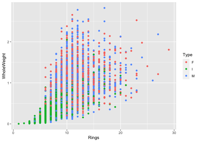
ggplot2
library(ggplot2)
# Total weigth in function of number of rings.
class(dset_dt)

## [1] "data.table" "data.frame"

ggplot(dset_dt, aes(x = Rings, y = WholeWeight, color = Type)) +
  geom_point()
 ### with the tidyverse
library("tidyverse")

## ── Attaching packages ─────────────────────────────────────── tidyverse 1.3.0 ──

## ✓ tibble  3.0.4     ✓ dplyr   1.0.2
## ✓ tidyr   1.1.2     ✓ stringr 1.4.0
## ✓ readr   1.4.0     ✓ forcats 0.5.0
## ✓ purrr   0.3.4

## ── Conflicts ────────────────────────────────────────── tidyverse_conflicts() ──
## x dplyr::between()   masks data.table::between()
## x dplyr::filter()    masks stats::filter()
## x dplyr::first()     masks data.table::first()
## x dplyr::lag()       masks stats::lag()
## x dplyr::last()      masks data.table::last()
## x purrr::transpose() masks data.table::transpose()

class(dset_dt)

## [1] "data.table" "data.frame"

dset_dt %>%
  filter(Type == "M") # But this doesn't run faster than a data frame.

##         V1 Type LongestShell   Dia Height WholeWeight ShuckedWeight
##    1:  521    M        0.210 0.150  0.050      0.0385        0.0155
##    2:  527    M        0.155 0.110  0.040      0.0155        0.0065
##    3: 2372    M        0.180 0.125  0.050      0.0230        0.0085
##    4:  519    M        0.325 0.230  0.090      0.1470        0.0600
##    5:  525    M        0.235 0.160  0.060      0.0545        0.0265
##   ---
## 1524: 2336    M        0.610 0.490  0.150      1.1030        0.4250
## 1525: 2437    M        0.515 0.400  0.160      0.8175        0.2515
## 1526: 3281    M        0.690 0.540  0.185      1.6195        0.5330
## 1527:  295    M        0.600 0.495  0.195      1.0575        0.3840
## 1528: 2109    M        0.665 0.535  0.225      2.1835        0.7535
##       VisceraWeight ShellWeight Rings Masse_Tot2   Masse_Tot3 Masse_Tot4   ID
##    1:        0.0085       0.010     3     0.0340 1.317500e-06    -0.0030    6
##    2:        0.0030       0.005     3     0.0145 9.750000e-08    -0.0015    7
##    3:        0.0055       0.010     3     0.0240 4.675000e-07    -0.0070   13
##    4:        0.0340       0.045     4     0.1390 9.180000e-05    -0.0190   26
##    5:        0.0095       0.015     4     0.0510 3.776250e-06     0.0020   27
##   ---
## 1524:        0.2025       0.360    23     0.9875 3.098250e-02    -0.1375 4169
## 1525:        0.1560       0.300    23     0.7075 1.177020e-02    -0.2045 4170
## 1526:        0.3530       0.555    24     1.4410 1.044227e-01    -0.3750 4172
## 1527:        0.1900       0.375    26     0.9490 2.736000e-02    -0.1810 4174
## 1528:        0.3910       0.885    27     2.0295 2.607374e-01    -0.5225 4175
The vroom package
Introduction
Now that we know how to rapidly manipulate heavy data, let’s see how we can manipulate heavier data even faster. This is the idea behind the vroom package who’s objective is to maximize read and write spead by using an efficient parsing system that doesn’t load data in memory, but instead focuses on their structure.
What vroom does :
The main vroom function is vroom() and it is used to read databases
very fast, whatever their type, even if it’s compressed. It also
recognizes the data separation used in the files.
It contains almost all parsing functions contained in readr, but using multiple cores makes it much faster.
Differences with data.table :
The main difference between those two packages is the read speed, but
this is depends on the type of data. vroom will read character data
much faster than data.table but will be slower for pure numerical
datasets. Why? Because it indexes data at importation, and it is much
harder to index numerical values than characters, which are more
limited.
vroom also uses a different syntax to data.table, more fitting the the “tidy” writing of dplyr.
How does it work ? Concept behind vroom’s speed :
Vroom uses the Altrep (alternative representation) framework of R (only
for R 3.5+). This context allows a better management of memory during
heavy tasks. When importing files, the data is not stored in memory.
Vroom instead created a path (index) to find the data easily. Then, when
we apply a command, we only require the necessary data without reading
the whole dataset (on demand parsing). By mapping data and the memory,
vroom can perform multi-threaded analysis, giving big performance gains
even to laptops. The capacity of reading and writing strings in a
multi-threaded environment generates major speed improvement compared to
classic methods (see Jim Hester’s figure in the youtube reference below
@ 4:39). When multiple character vectors have the same name, they are
not stored multiple times, they are instead indexed in a way that allow
multiple path to lead to the same object. This greatly diminishes memory
costs.
With both packages, we can then explore all types of data at high speed.
Installation
Vroom can be installed directly from CRAN or Github to obtain latest updates in the package.
# CRAN
install.packages("vroom")

# GitHub
devtools::install_dev("vroom")

library(vroom) # load the package
Reading data
Single file
Let’s import the abalone dataset again, containing mostly characters and numerical variables.
vab <- vroom("abalone.csv")

## New names:
## * `` -> ...1

## Rows: 4,177
## Columns: 10
## Delimiter: ","
## chr [1]: Type
## dbl [9]: ...1, LongestShell, Diameter, Height, WholeWeight, ShuckedWeight, VisceraWeight...
##
## Use `spec()` to retrieve the guessed column specification
## Pass a specification to the `col_types` argument to quiet this message
The output is a 4 177 x 9 tibble delimited by “;” separator.
While the function can guess the type of separator, it can make mistakes. It must then be specified using the delim = [either(“,” “” “ “|” “:” “;”)] argument. It is a better practice to specify it manually, resulting in additionnal speed gains.
Vroom also guesses column type, so it might be necessary to specify column format.
vab <- vroom("abalone.csv", delim = ",")

## New names:
## * `` -> ...1

## Rows: 4,177
## Columns: 10
## Delimiter: ","
## chr [1]: Type
## dbl [9]: ...1, LongestShell, Diameter, Height, WholeWeight, ShuckedWeight, VisceraWeight...
##
## Use `spec()` to retrieve the guessed column specification
## Pass a specification to the `col_types` argument to quiet this message
Let’s see the time difference between both methods.
system.time({t_ab <- vroom("abalone.csv")})

## New names:
## * `` -> ...1

## Rows: 4,177
## Columns: 10
## Delimiter: ","
## chr [1]: Type
## dbl [9]: ...1, LongestShell, Diameter, Height, WholeWeight, ShuckedWeight, VisceraWeight...
##
## Use `spec()` to retrieve the guessed column specification
## Pass a specification to the `col_types` argument to quiet this message

##    user  system elapsed
##   0.022   0.002   0.023

system.time({t_abdelim <- vroom("abalone.csv", delim = ",")})

## New names:
## * `` -> ...1
## Rows: 4,177
## Columns: 10
## Delimiter: ","
## chr [1]: Type
## dbl [9]: ...1, LongestShell, Diameter, Height, WholeWeight, ShuckedWeight, VisceraWeight...
##
## Use `spec()` to retrieve the guessed column specification
## Pass a specification to the `col_types` argument to quiet this message

##    user  system elapsed
##   0.018   0.002   0.017
And now the read time difference between data.table and vroom for the database created previously, “m2.csv” .
system.time({dt_m2 <- fread("m2.csv")})

##    user  system elapsed
##   0.050   0.024   0.174

system.time({v_m2 <- vroom("m2.csv", delim = ",")})

## Rows: 1,000,000
## Columns: 1
## Delimiter: ","
## dbl [1]: matrix.runif.1e.06...nrow...1e.06.
##
## Use `spec()` to retrieve the guessed column specification
## Pass a specification to the `col_types` argument to quiet this message

##    user  system elapsed
##   0.064   0.009   0.026
- If we use “;” the columns will be “chr” and “,” for “dbl”
Multiple files
Vroom can also read multiple dataset with the same column names and combine them into a single database. Let’s use a copy of abalone.csv for example.
file.copy("abalone.csv","abalone_copy.csv") # copy abalone.csv to abalone_copy.csv

## [1] TRUE

library("fs")

files <- dir_ls(glob = "abalone*csv") # Seeks all files containing abalone and csv in the working directory

files

## abalone.csv      abalone_copy.csv

vroom(files, delim = ",") # Imports both files as a single dataset

## New names:
## * `` -> ...1

## Rows: 8,354
## Columns: 10
## Delimiter: ","
## chr [1]: Type
## dbl [9]: ...1, LongestShell, Diameter, Height, WholeWeight, ShuckedWeight, VisceraWeight...
##
## Use `spec()` to retrieve the guessed column specification
## Pass a specification to the `col_types` argument to quiet this message

## # A tibble: 8,354 x 10
##     ...1 Type  LongestShell Diameter Height WholeWeight ShuckedWeight
##    <dbl> <chr>        <dbl>    <dbl>  <dbl>       <dbl>         <dbl>
##  1     1 M            0.455    0.365  0.095       0.514        0.224
##  2     2 M            0.35     0.265  0.09        0.226        0.0995
##  3     3 F            0.53     0.42   0.135       0.677        0.256
##  4     4 M            0.44     0.365  0.125       0.516        0.216
##  5     5 I            0.33     0.255  0.08        0.205        0.0895
##  6     6 I            0.425    0.3    0.095       0.352        0.141
##  7     7 F            0.53     0.415  0.15        0.778        0.237
##  8     8 F            0.545    0.425  0.125       0.768        0.294
##  9     9 M            0.475    0.37   0.125       0.509        0.216
## 10    10 F            0.55     0.44   0.15        0.894        0.314
## # … with 8,344 more rows, and 3 more variables: VisceraWeight <dbl>,
## #   ShellWeight <dbl>, Rings <dbl>
To differenciate between different data sources it is possible to add the “id=” argument to add a column refering to the original file.
m_vab <- vroom(files, delim = ",", id = "source")

## New names:
## * `` -> ...1

## New names:
## * ...1 -> ...2

## Rows: 8,354
## Columns: 11
## Delimiter: ","
## chr [1]: Type
## dbl [9]: ...1, LongestShell, Diameter, Height, WholeWeight, ShuckedWeight, VisceraWeight...
##
## Use `spec()` to retrieve the guessed column specification
## Pass a specification to the `col_types` argument to quiet this message

head(m_vab)

## # A tibble: 6 x 11
##   source  ...2 Type  LongestShell Diameter Height WholeWeight ShuckedWeight
##   <chr>  <dbl> <chr>        <dbl>    <dbl>  <dbl>       <dbl>         <dbl>
## 1 abalo…     1 M            0.455    0.365  0.095       0.514        0.224
## 2 abalo…     2 M            0.35     0.265  0.09        0.226        0.0995
## 3 abalo…     3 F            0.53     0.42   0.135       0.677        0.256
## 4 abalo…     4 M            0.44     0.365  0.125       0.516        0.216
## 5 abalo…     5 I            0.33     0.255  0.08        0.205        0.0895
## 6 abalo…     6 I            0.425    0.3    0.095       0.352        0.141
## # … with 3 more variables: VisceraWeight <dbl>, ShellWeight <dbl>, Rings <dbl>
Compressed files
To read compressed files, the same method is used, but adding the appropriate extension at the end of the file names. i.e.: vroom(“abalone.csv.gz”)
Other filetypes
Vroom can also read multiple compressed files (wrapper function), files from online sources (put the URL in vroom) and compressed files from online sources. We invite you to refer to this tutorial which this workshop is based upon for more information : (https://vroom.r-lib.org/articles/vroom.html)
Manipulating data
Selecting columns
Column selection is made in a similar fashion to “dplyr” using the col_select=c() argument. It can be donne by column type, or by string match (starts with “T”, ends with “e”, etc.)
head(vroom("abalone.csv", col_select = c(Type, Rings, WholeWeight)))

## New names:
## * `` -> ...1

## # A tibble: 6 x 3
##   Type  Rings WholeWeight
##   <chr> <dbl>       <dbl>
## 1 M        15       0.514
## 2 M         7       0.226
## 3 F         9       0.677
## 4 M        10       0.516
## 5 I         7       0.205
## 6 I         8       0.352

head(vroom("abalone.csv", col_select = c(1, 5, 9)))

## New names:
## * `` -> ...1

## # A tibble: 6 x 3
##    ...1 Height ShellWeight
##   <dbl>  <dbl>       <dbl>
## 1     1  0.095       0.15
## 2     2  0.09        0.07
## 3     3  0.135       0.21
## 4     4  0.125       0.155
## 5     5  0.08        0.055
## 6     6  0.095       0.12

head(vroom("abalone.csv", col_select = starts_with("T")))

## New names:
## * `` -> ...1

## # A tibble: 6 x 1
##   Type
##   <chr>
## 1 M
## 2 M
## 3 F
## 4 M
## 5 I
## 6 I

head(vroom("abalone.csv", col_select = ends_with("ght")))

## New names:
## * `` -> ...1

## # A tibble: 6 x 5
##   Height WholeWeight ShuckedWeight VisceraWeight ShellWeight
##    <dbl>       <dbl>         <dbl>         <dbl>       <dbl>
## 1  0.095       0.514        0.224         0.101        0.15
## 2  0.09        0.226        0.0995        0.0485       0.07
## 3  0.135       0.677        0.256         0.142        0.21
## 4  0.125       0.516        0.216         0.114        0.155
## 5  0.08        0.205        0.0895        0.0395       0.055
## 6  0.095       0.352        0.141         0.0775       0.12
Renaming columns
Changing column names is less intuitive than with data.table.
vroom("abalone.csv", col_select = list(Sexe = Type, Dia = Diameter, everything())) # "everything()" selects all other variables (info @ ?everything()).

## New names:
## * `` -> ...1

## # A tibble: 4,177 x 10
##    Sexe    Dia  ...1 LongestShell Height WholeWeight ShuckedWeight VisceraWeight
##    <chr> <dbl> <dbl>        <dbl>  <dbl>       <dbl>         <dbl>         <dbl>
##  1 M     0.365     1        0.455  0.095       0.514        0.224         0.101
##  2 M     0.265     2        0.35   0.09        0.226        0.0995        0.0485
##  3 F     0.42      3        0.53   0.135       0.677        0.256         0.142
##  4 M     0.365     4        0.44   0.125       0.516        0.216         0.114
##  5 I     0.255     5        0.33   0.08        0.205        0.0895        0.0395
##  6 I     0.3       6        0.425  0.095       0.352        0.141         0.0775
##  7 F     0.415     7        0.53   0.15        0.778        0.237         0.142
##  8 F     0.425     8        0.545  0.125       0.768        0.294         0.150
##  9 M     0.37      9        0.475  0.125       0.509        0.216         0.112
## 10 F     0.44     10        0.55   0.15        0.894        0.314         0.151
## # … with 4,167 more rows, and 2 more variables: ShellWeight <dbl>, Rings <dbl>
If we want to modify all column names so they have a similar format without doing so manually (notably in excel, which is a big no with Big Data), you can use the “.name_repair=” argument from the janitor package
install.packages("janitor")

library("janitor")

##
## Attaching package: 'janitor'

## The following objects are masked from 'package:stats':
##
##     chisq.test, fisher.test

head(vroom("abalone.csv", .name_repair = ~ make_clean_names(., case = "all_caps")))

## Rows: 4,177
## Columns: 10
## Delimiter: ","
## chr [1]: TYPE
## dbl [9]: X, LONGEST_SHELL, DIAMETER, HEIGHT, WHOLE_WEIGHT, SHUCKED_WEIGHT, VISCERA_WEIGH...
##
## Use `spec()` to retrieve the guessed column specification
## Pass a specification to the `col_types` argument to quiet this message

## # A tibble: 6 x 10
##       X TYPE  LONGEST_SHELL DIAMETER HEIGHT WHOLE_WEIGHT SHUCKED_WEIGHT
##   <dbl> <chr>         <dbl>    <dbl>  <dbl>        <dbl>          <dbl>
## 1     1 M             0.455    0.365  0.095        0.514         0.224
## 2     2 M             0.35     0.265  0.09         0.226         0.0995
## 3     3 F             0.53     0.42   0.135        0.677         0.256
## 4     4 M             0.44     0.365  0.125        0.516         0.216
## 5     5 I             0.33     0.255  0.08         0.205         0.0895
## 6     6 I             0.425    0.3    0.095        0.352         0.141
## # … with 3 more variables: VISCERA_WEIGHT <dbl>, SHELL_WEIGHT <dbl>,
## #   RINGS <dbl>
Adding new columns
For other types of data manipulations, it is possible to use dplyr normally, since the object format generated by vroom are compatible with dplyr. As opposed to manipulations done with vroom where we need to include the original file path, dplyr must refer to the imported object in the R environment.
library("dplyr")
test = mutate(vab, new = WholeWeight/Diameter)
head(test)

## # A tibble: 6 x 11
##    ...1 Type  LongestShell Diameter Height WholeWeight ShuckedWeight
##   <dbl> <chr>        <dbl>    <dbl>  <dbl>       <dbl>         <dbl>
## 1     1 M            0.455    0.365  0.095       0.514        0.224
## 2     2 M            0.35     0.265  0.09        0.226        0.0995
## 3     3 F            0.53     0.42   0.135       0.677        0.256
## 4     4 M            0.44     0.365  0.125       0.516        0.216
## 5     5 I            0.33     0.255  0.08        0.205        0.0895
## 6     6 I            0.425    0.3    0.095       0.352        0.141
## # … with 4 more variables: VisceraWeight <dbl>, ShellWeight <dbl>, Rings <dbl>,
## #   new <dbl>
Writing data
Writing files is done in the same way as the reading, specifying the delimiters and the desired extention into the vroom_write() function.
vroom_write(vab, "vroom_abalone.csv", delim = ";")
To make a compressed file, simply add a second extension:
vroom_write(vab, "vroom_abalone.csv.gz")
References
About Big Data: https://www.environmentalscience.org/data-science-big-data https://click.endnote.com/viewer?doi=10.1890%2F120103&token=WzI0OTgxMjksIjEwLjE4OTAvMTIwMTAzIl0.94jMXqxm3lJEzbuAhWEzvzal-xI
Data.table:
https://www.listendata.com/2016/10/r-data-table.html
https://www.datacamp.com/community/tutorials/top-ten-most-important-packages-in-r-for-data-science
https://www.machinelearningplus.com/data-manipulation/datatable-in-r-complete-guide/.
Keys:
https://cran.r-project.org/web/packages/data.table/vignettes/datatable-keys-fast-subset.html
Vroom:
https://vroom.r-lib.org/articles/vroom.html
Jim Hester:
https://www.youtube.com/watch?v=RA9AjqZXxMU&t=10s
https://vroom.r-lib.org/articles/benchmarks.html
Other filetypes:
https://vroom.r-lib.org/articles/vroom.html