Boruta Algorithm
Jade Dormoy-Boulanger
April 2025
- Step 1: Data Check
- Step 2: The test with a categorical response value (landuse)
- Step 3: Results visualization
- Step 4: The test with numerical value response (zinc)
- Step 5: Results visualization
The Boruta algorithm is a machine learning feature selection tool designed to select significant explicative values for a given model. Boruta is also a wrapper algorithm around Random Forests trees, meaning it uses the Random Forest trees classification method to train and evaluate a predictive model. Fun fact: “Boruta” comes from the slave mythology where Boruta is a forest spirit.
The Boruta algorithm aims to provide a stable and ranked selection of important and non-important factors. To achieve this it compares median Z scores of the provided values for a given model to those of “shadow” features (features based on a strictly random distribution).
This algorithm offers several very interesting characteristics for disciplines related to environmental science :
- Can be used with both continuous and categorical variables
- Due to its iterative nature, it deals well with correlations between explanatory variables (No need to care for this anymore!)
- It ranks the significant factors found
- It is very efficient when there is a lot of explicative values
Boruta also has some negative points:
- It does not work well with NAs in a dataset
- It is a relatively slow process to execute, especially when it’s analyzing a big dataset
NB: Analysis presented into this tutorial make no sense on a scientific point of view. Theyr are just used as examples.
Now that we have a head round the Boruta algorithm, let’s try it!
#Packages' installation and loading
#install.packages(c("Boruta", "Amelia", "randomForest", "sp", "pdp"))
library(Boruta)
library(Amelia)
library(randomForest)
library(sp)
library(pdp)

#Data
data("meuse") # Dataset on heavy metal pollution in the Meuse floodplain, Netherlands
Step 1: Data Check
We need to check if our dataset has NAs and if categorical values are encoded as factors.
#Data check
str(meuse)  # Everything looks good, categorical values are factor encoded
'data.frame':	155 obs. of  14 variables:
 $ x      : num  181072 181025 181165 181298 181307 ...
 $ y      : num  333611 333558 333537 333484 333330 ...
 $ cadmium: num  11.7 8.6 6.5 2.6 2.8 3 3.2 2.8 2.4 1.6 ...
 $ copper : num  85 81 68 81 48 61 31 29 37 24 ...
 $ lead   : num  299 277 199 116 117 137 132 150 133 80 ...
 $ zinc   : num  1022 1141 640 257 269 ...
 $ elev   : num  7.91 6.98 7.8 7.66 7.48 ...
 $ dist   : num  0.00136 0.01222 0.10303 0.19009 0.27709 ...
 $ om     : num  13.6 14 13 8 8.7 7.8 9.2 9.5 10.6 6.3 ...
 $ ffreq  : Factor w/ 3 levels "1","2","3": 1 1 1 1 1 1 1 1 1 1 ...
 $ soil   : Factor w/ 3 levels "1","2","3": 1 1 1 2 2 2 2 1 1 2 ...
 $ lime   : Factor w/ 2 levels "0","1": 2 2 2 1 1 1 1 1 1 1 ...
 $ landuse: Factor w/ 15 levels "Aa","Ab","Ag",..: 4 4 4 11 4 11 4 2 2 15 ...
 $ dist.m : num  50 30 150 270 380 470 240 120 240 420 ...
meuse <- meuse[, -c(1,2)] # getting rid the coordinates, since we don't need them

#Checking for NAs
missmap(meuse) #We have NAs!
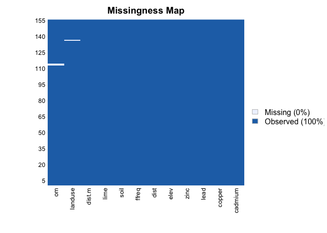
#getting rid if the missing data
meuse <- na.omit(meuse) # Usually, we would have taken care of it differently, but for this workshop it works

missmap(meuse) #everything's fine, we move forward!

Step 2: The test with a categorical response value (landuse)
set.seed(666) # Add some randomness and insure reproductive results

boruta.tree <- Boruta(landuse~.,meuse, doTrace = 2) # the test
getSelectedAttributes(boruta.tree, withTentative = F) #The results
 [1] "cadmium" "copper"  "lead"    "zinc"    "elev"    "dist"    "om"
 [8] "soil"    "lime"    "dist.m"
result.boruta <- attStats(boruta.tree) # saving the results within an object
result.boruta # everything is comfirmed except ffreq (flooding frequency)
         meanImp medianImp    minImp    maxImp  normHits  decision
cadmium 5.945723  6.014663 2.5914729  8.063450 0.9090909 Confirmed
copper  7.113778  7.175817 5.0427523  9.119944 0.9898990 Confirmed
lead    4.376747  4.469601 1.7236572  8.206230 0.8181818 Confirmed
zinc    5.406644  5.400178 2.5531753  7.955784 0.9292929 Confirmed
elev    6.195954  6.224019 2.5389805  9.282901 0.9595960 Confirmed
dist    8.247251  8.232837 5.6687932 10.814695 1.0000000 Confirmed
om      4.900863  4.892887 2.4107399  7.345374 0.8787879 Confirmed
ffreq   3.334017  3.227131 1.1318711  5.830546 0.6161616 Tentative
soil    3.819919  3.889711 2.0409078  7.229944 0.7474747 Confirmed
lime    3.606756  3.697002 0.6825293  5.498580 0.6767677 Confirmed
dist.m  8.362581  8.387298 5.7266492 10.785228 1.0000000 Confirmed
boruta.tree.2 <- TentativeRoughFix(boruta.tree)#classify tentatives

getSelectedAttributes(boruta.tree.2, withTentative = F)#new results
 [1] "cadmium" "copper"  "lead"    "zinc"    "elev"    "dist"    "om"
 [8] "ffreq"   "soil"    "lime"    "dist.m"
result.boruta <- attStats(boruta.tree.2)
result.boruta # Finally, everything is significant at explaining landuse
         meanImp medianImp    minImp    maxImp  normHits  decision
cadmium 5.945723  6.014663 2.5914729  8.063450 0.9090909 Confirmed
copper  7.113778  7.175817 5.0427523  9.119944 0.9898990 Confirmed
lead    4.376747  4.469601 1.7236572  8.206230 0.8181818 Confirmed
zinc    5.406644  5.400178 2.5531753  7.955784 0.9292929 Confirmed
elev    6.195954  6.224019 2.5389805  9.282901 0.9595960 Confirmed
dist    8.247251  8.232837 5.6687932 10.814695 1.0000000 Confirmed
om      4.900863  4.892887 2.4107399  7.345374 0.8787879 Confirmed
ffreq   3.334017  3.227131 1.1318711  5.830546 0.6161616 Confirmed
soil    3.819919  3.889711 2.0409078  7.229944 0.7474747 Confirmed
lime    3.606756  3.697002 0.6825293  5.498580 0.6767677 Confirmed
dist.m  8.362581  8.387298 5.7266492 10.785228 1.0000000 Confirmed
median<-data.frame(boruta.tree$ImpHistory)# important data to report the results. usually we report the significant factors found as well as the algorithm success (% of significant factors found compared to the number of factor entered into the model initially)

median(median$shadowMax)
[1] 2.747589
median(median$shadowMin)
[1] -2.562369
median(median$shadowMean)
[1] -0.1019566
median(median$cadmium)
[1] 6.014663
median(median$copper)
[1] 7.175817
median(median$lead)
[1] 4.469601
median(median$zinc)
[1] 5.400178
#etc...
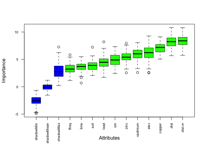
Step 3: Results visualization
plot(boruta.tree.2, las = 2, cex.axis = 0.7) # red = rejected, blue = shadow, shadow = significant (the most important one is dist.m, the distance from the Meuse in meter)
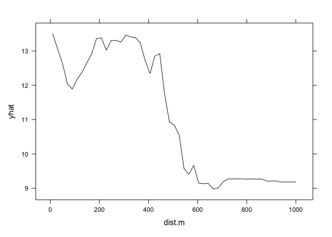
#Now, what is the distance impact on the landuse?
#We will use a partial dependency plot

landuse<- randomForest(landuse~ ., meuse, importance = T) # we add the significant values found significant

graph.landuse<- pdp::partial(landuse,pred.var = "dist.m", which.class = "W", plot=F)#generate the plot data for pasture
pdp::plotPartial(graph.landuse) # the plot, yhat = pasture probability, from 500 m and further away from the Meuse, We have drastically less probabilities of having a pasture
And what if we would like to plot a categorical explicative value? Let’s try with soil types
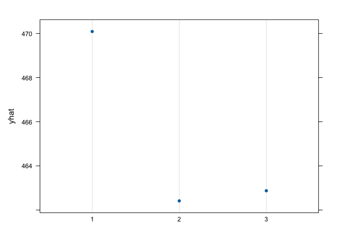
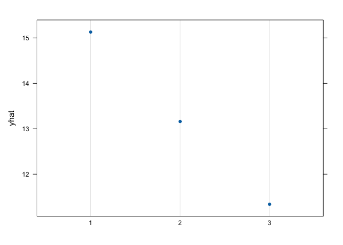
graph.landuse<- pdp::partial(landuse,pred.var = "soil", which.class = "W", plot=F) #generate the plot data for pasture
pdp::plotPartial(graph.landuse) # the plot, yhat = pasture probability, we have more probabilities of finding pastures in a calcareous soil, followed by non-calcareous and red brick soils
Step 4: The test with numerical value response (zinc)
set.seed(666) # Add some randomness and insure reproductive results

boruta.tree <- Boruta(zinc~.,meuse, doTrace = 2) # the test
getSelectedAttributes(boruta.tree, withTentative = F) #the results
 [1] "cadmium" "copper"  "lead"    "elev"    "dist"    "om"      "ffreq"
 [8] "soil"    "lime"    "dist.m"
result.boruta <- attStats(boruta.tree) # saving the results within an object
result.boruta # Everything is confirmed except landuse
          meanImp medianImp     minImp    maxImp  normHits  decision
cadmium 16.458307 16.394723 14.7122498 18.051753 1.0000000 Confirmed
copper  15.555833 15.511075 13.8689020 17.444924 1.0000000 Confirmed
lead    21.253972 21.226569 19.6326531 23.940836 1.0000000 Confirmed
elev     9.001595  9.048899  7.6848202 10.376720 1.0000000 Confirmed
dist    10.737130 10.792605  9.0666052 12.261163 1.0000000 Confirmed
om       8.033467  8.042202  6.8227216  9.728283 1.0000000 Confirmed
ffreq    5.382730  5.378091  4.1323604  6.818991 1.0000000 Confirmed
soil     5.301180  5.349173  3.9041242  6.643438 1.0000000 Confirmed
lime     6.183204  6.203087  4.7119003  7.519099 1.0000000 Confirmed
landuse  1.895212  1.883330 -0.2597717  3.966757 0.4444444 Tentative
dist.m   9.983445  9.973984  8.4906941 11.464105 1.0000000 Confirmed
boruta.tree.2 <- TentativeRoughFix(boruta.tree)

result.boruta <- attStats(boruta.tree.2) # saving the results within an object
result.boruta
          meanImp medianImp     minImp    maxImp  normHits  decision
cadmium 16.458307 16.394723 14.7122498 18.051753 1.0000000 Confirmed
copper  15.555833 15.511075 13.8689020 17.444924 1.0000000 Confirmed
lead    21.253972 21.226569 19.6326531 23.940836 1.0000000 Confirmed
elev     9.001595  9.048899  7.6848202 10.376720 1.0000000 Confirmed
dist    10.737130 10.792605  9.0666052 12.261163 1.0000000 Confirmed
om       8.033467  8.042202  6.8227216  9.728283 1.0000000 Confirmed
ffreq    5.382730  5.378091  4.1323604  6.818991 1.0000000 Confirmed
soil     5.301180  5.349173  3.9041242  6.643438 1.0000000 Confirmed
lime     6.183204  6.203087  4.7119003  7.519099 1.0000000 Confirmed
landuse  1.895212  1.883330 -0.2597717  3.966757 0.4444444  Rejected
dist.m   9.983445  9.973984  8.4906941 11.464105 1.0000000 Confirmed
median<-data.frame(boruta.tree.2$ImpHistory)# important data to report the results. usually we report the significant factors found as well as the algorithm success (% of significant factors found compared to the number of factor entered into the model initially)

median(median$shadowMax)
[1] 2.116256
median(median$shadowMin)
[1] -2.019417
median(median$shadowMean)
[1] -0.06191307
median(median$cadmium)
[1] 16.39472
median(median$copper)
[1] 15.51107
median(median$lead)
[1] 21.22657
median(median$elev)
[1] 9.048899
#etc...
Step 5: Results visualization
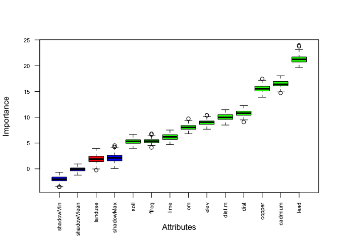
plot(boruta.tree.2, las = 2, cex.axis = 0.7) # red = rejected, blue = shadow, green= significant (the most important one is lead concentration)
#Now, what is the lead concentration impact on the zinc?
#We will use a partial dependency plot
zinc <- randomForest(zinc ~ cadmium + copper + lead + elev +
dist + om + ffreq + soil + lime, meuse, importance = T)# adding the significant factors found
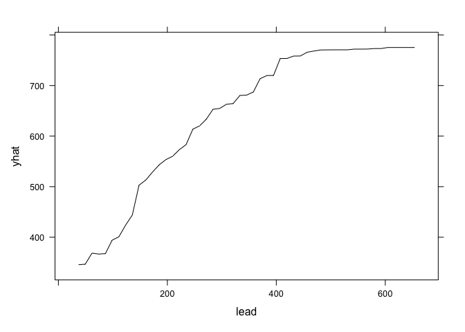
graph.zinc<- pdp::partial(zinc,pred.var = "lead", plot=F) #generate the plot data
pdp::plotPartial(graph.zinc) # the plot, yhat = zinc probability, the highest is the lead, the highest is the zinc
And what if we would like to plot a categorical explicative value? Let’s try with the soil type
graph.zinc<- pdp::partial(zinc,pred.var = "soil", plot=F) #generate the plot data
pdp::plotPartial(graph.zinc) # the plot, yhat = zinc probability, calcareous soils are the most zinc contaminated