Introduction to Deep Learning for Ecologists
Charles Martin
July 2021
- Introduction
- The bits and pieces of DL
- Doing DL in R
- Overfitting and underfitting
- Data considerations
- Wait, what’s a tensor?
- A basic example
- How do computers see ?
- ConvNets explained
- An image classification example
- Advanced techniques
- Typical workflow
- References
Introduction
Hi everyone. Welcome to this second Numerilab workshop on machine learning, this time aimed to introduce you to deep learning techniques with the Keras library.
First of all, let’s go over some definitions so we all are speaking with the vocabulary. And, bear in mind, there is some confusion floating around about these terms, so you might find different definitions elsewhere.
Usually, when we talk about Artificial Intelligence (AI), we talk about any technique where the computer does something for us, in a automated way. It is a very broad term.
More specifically, one can talk about Machine Learning (ML), where you present the computer with some inputs and expected outputs, and the software finds the best set of rules of map between the two. Your usual ecological stats techniques fall into this definition, namely regression and ANOVA, but also classification trees, random forests, etc.
Finally, when one talks about Deep Learning (DL), we usually talk about very specific ML techniques, where data representations (think like a PCA for example) are connected together in successive layers, usually with what we call Neural Networks (NN).
Contrary to popular belief, the deep in DL has nothing to do with profound learning. It only acknowledges that there are many layers of information representation stacked onto one another.
While we are at it, let’s tackle another myth. You might have heard that NN process information just like the cells in the brain would. This is mostly incorrect. The processes in the brain are much more complex than what we’re building today. So, you’ll do yourself a great service by not thinking about DL as a brain, but mostly as an advanced ML algorithm that has many tricks to represent information in interesting ways. In fact, the breakthroughs DL have made so far are mostly what expert calls highly perceptual tasks like image and recognition, where data representations are highly complex (i.e. difficult to fit into a rectangle matrix).
As this workshop is mostly on an advanced topic (I’ll still try to keep things as simple as possible for you), it assumes you know the basics of data visualization and manipulation in R. Ideally, you will also be familiar with some basic ML concepts, but I’ll try to explain these ideas as we go.
If you need a refresher on these topics, take a quick glance here :
- https://rive-numeri-lab.github.io/workshops/RapidDataViz
- https://rive-numeri-lab.github.io/workshops/RapidDataManip
The bits and pieces of DL
So then, what is a DL model? How does it work?
Architecture
As we said above, DL models try to find the best mapping possible between inputs and outputs. In DL parlance, these outputs are called usually targets.
The inputs are fed into a first layer of transformations, the output of which is fed to the second layer and so on, until the last layer of the model, which predicts a target value for the given input.
Each layer contains a series of weights, just like in regression or PCA, that are used to map inputs to outputs. But unlike regression or PCA, DL models can (and will) contain millions of such weights to optimize.
Two important functions
But before getting into the optimization part, we have to define how our DL model
measures how close it is to the actual target values.
We’ll call that the loss function
(you’ll also see sometimes the term objective function).
In the classic regression model,
the loss function would be (the mean squared error).
Since DL models are much more versatile, you have many more options.
For regression-type problems, you’ll indeed use the mean-squared error,
but for two-class classification problems, you’ll use binary cross-entropy,
for many-class problems categorical cross-entropy, etc.
Cross-entropy you say? As of now, it is not that important to understand the intricate Information Theory details here. You can think of binary cross-entropy as a binary version of the mean-squared error, where the distances from a predicted probability farther from 1 (full certainty) are exponentially penalized.
Once our DL knows how far from its target it is, it needs a way to change its set of weights to try to get closer to the target. Usually, when one talks about DL models, it is assumed that the optimizing function is some form of Stochastic Gradient Descent (SGD). In a simple one-parameter context, SGD tries to determine the gradient around its current point, by moving the parameter value a little on either side of its current value. It would then choose which way improves its loss function the most and move the parameter value an arbitrary amount (the learning rate) to that side. It would then repeat that process until it reaches a point where the loss function cannot be improved anymore.
In a complex thousands-of-parameters model, things can get a little more complicated(!), but luckily for you, clever computer scientists have discovered a way to implement such strategies efficiently in a neural network with an algorithm called backpropagation. We won’t go into the details of this algorithm here. Suffice to know that it is more or less the breakthrough that allowed the field of DL to exist. Many implementations of this backpropagation algorithm exist, but unless you are going into uncharted territory, the rmsprop optimizer will be your best bet when choosing your optimizer function.
What’s in a layer?
Finally, the last bit of information we need to understand before delving into the code is : what’s going on inside a neural network layer?
A layer is defined by 3 things : its inputs, its hidden units, and its outputs. In a densely connected layer (i.e. most layers we will see today), each hidden unit receives every input value, and every hidden unit is connected to every output value.
So, for example, if we defined our layer as having 3 input values, 3 hidden units and 2 output values, each of the 3 hidden units will receive 3 inputs to make its calculation. Also, 2 output computations will receive each 3 values to make their calculations.

And here is another key aspect that makes DL models click : instead of using linear combinations to make their calculations, DL models use non-linear activation functions. The reason for that is that it opens-up the representation space to which the DL model has access, to the contrary of stacking layers of linear transformations, which would not open-up the hypothesis space. There are a plethora of activation function available for this purpose, the most common for hidden layers being the relu function (for Rectified Linear Unit), which has a flat part, and a slope part :

You’ll also see that at the end of the stack, you’ll use different kinds of activation function, for example the sigmoid function for probabilities, or simply no activation function at all for the output of regression problems.
Doing DL in R
Keras installation
So, now that your head is spinning with new words and concepts, let’s get back down to earth and start doing.
As of now, there is no contest that the best DL library on the market is Keras. Almost every DL tutorial or book you’ll find uses this library. The major hurdle for us today though, is that Keras is built with Python code, whereas our workshops usually assume you are working with R. Hopefully, you won’t have to learn Python today, as there exists an R library that allows us to use the Keras code inside our R environment. Although it is a neat little trick to do that, it also complicates the installation process a bit.
Upon installing the keras package in the usual way, you’ll have additional steps to complete before getting to work.
So, the usual installation step is :
install.packages("keras")
You then activate the package :
library(keras)
Then, as Keras is a Python library we’ll call from R, you need to also install a Python interpreter. If you’re on Windows, the simplest solution is to install Anaconda (https://www.anaconda.com/download/#windows), which is a Python distribution, bundled with library management tools, etc.
Once Anaconda (and thus Python) is installed, you also need to install the Keras library per se, as the R package doesn’t contain Keras code, only code to manipulate the Python library.
To install the actual Keras code, you’ll need to run :
install_keras()
This command might take a while (i.e. many minutes),
Please note that, after install_keras has been run successfully once, you don’t need to run it again (just like package your usual installations). Only running
library(keras)
will be sufficient.
Hello World - testing your installation
As the Keras installation process can be a perilous adventure, I strongly suggest you copy-paste this small test code, just to make sure everything is working correctly :
mnist <- dataset_mnist()
x_train <- mnist$train$x
y_train <- mnist$train$y
x_test <- mnist$test$x
y_test <- mnist$test$y

# reshape
x_train <- array_reshape(x_train, c(nrow(x_train), 784))
x_test <- array_reshape(x_test, c(nrow(x_test), 784))
# rescale
x_train <- x_train / 255
x_test <- x_test / 255

y_train <- to_categorical(y_train, 10)
y_test <- to_categorical(y_test, 10)

model <- keras_model_sequential() %>%
  layer_dense(units = 256, activation = 'relu', input_shape = c(784)) %>%
  layer_dropout(rate = 0.4) %>%
  layer_dense(units = 128, activation = 'relu') %>%
  layer_dropout(rate = 0.3) %>%
  layer_dense(units = 10, activation = 'softmax')

summary(model)
Model: "sequential"
________________________________________________________________________________
Layer (type)                        Output Shape                    Param #
================================================================================
dense_2 (Dense)                     (None, 256)                     200960
________________________________________________________________________________
dropout_1 (Dropout)                 (None, 256)                     0
________________________________________________________________________________
dense_1 (Dense)                     (None, 128)                     32896
________________________________________________________________________________
dropout (Dropout)                   (None, 128)                     0
________________________________________________________________________________
dense (Dense)                       (None, 10)                      1290
================================================================================
Total params: 235,146
Trainable params: 235,146
Non-trainable params: 0
________________________________________________________________________________
model %>% compile(
  loss = 'categorical_crossentropy',
  optimizer = optimizer_rmsprop(),
  metrics = c('accuracy')
)

history <- model %>% fit(
  x_train, y_train,
  epochs = 15, batch_size = 128,
  validation_split = 0.2
)

plot(history)
`geom_smooth()` using formula 'y ~ x'
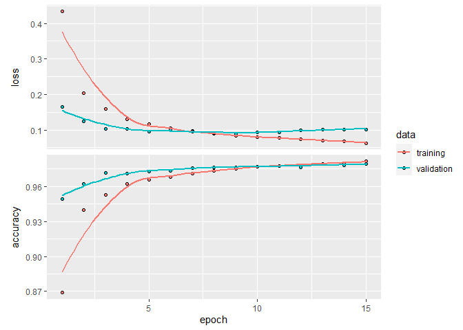
model %>% evaluate(x_test, y_test)
      loss   accuracy
0.09015266 0.98110002
model %>% predict_classes(x_test[1:5,])
[1] 7 2 1 0 4
This code might take a couple of minutes to run, as it is learning to recognize hand-written digits! It is the Hello World of DL. We won’t delve into that example here, but you can read more about the particular problem in many places on the web, e.g. here https://tensorflow.rstudio.com/guide/keras/.
About Python error messages
As you’ll move along on your DL voyage, you’ll encounter many cryptic error messages. Moreso than with any other R packages you’ve tried. That is because the errors are coming from the Python code, which your R code is calling. They will often be cryptic and unhelpful, and if you ask me : it is the major pain point of this approach.
In the trials and errors preceding the writing of this workshop, I realized that the two recurring errors I was facing were that :
(1) My data was not in a matrix format. Contrary to most R libraries that work seamlessly with either data.frame, tibble, or matrix objects, Keras needs you data to be in matrices, but the error won’t tell you that exactly.
(2) My data was not in the same dimensions as the input layer of my DL model. Again, the error is some internal Python error code and note a simple “mismatch between data matrix and model definition”. That would have been too easy I guess.
Overfitting and underfitting
One concept that is especially important to understand when working on ML problems is the concept of underfitting and overfitting. We say that an model is underfitted when it is not extracting the maximum possible out of our data. An underfitted model could make better predictions if it had more parameters, more interactions, more time to learn, etc. On the other hand, an overfitted model knows our training data a little too well. It performs very well on the training data, but fails miserably when presented with new data. It does not generalize well outside of what was presented to it.
It is a dilemma that must always be kept in mind when attacking ML problems.
Data considerations
There are many levels at which we can avoid this overfitting problem. Some of which we’ll cover here, others we’ll cover later once we have seen the specifics of DL models.
First of all, when preparing our dataset. You need to make sure that your data is varied enough, i.e. that it shows enough of the expected variability of the natural phenomenon. DL models are VERY efficient, and will try any shortcut they can to improve their results.
They WILL recognize that you used a little “C” sticker on your control test tubes, or that you photographed control plots on a different, more cloudy day than your experimental treatments, etc. These considerations are even more important when working with human subjects. Having only pictures of your white-skinned friends in your dataset could prove awkward once you try your model on photos of black-skinned people and they end up being classified as gorillas. And before you start ridiculing my example, please know that it is actually a true story that happened at Google Photos (https://www.bbc.com/news/technology-33347866).
The second strategy to reduce the overfitting in our model is to make sure that we are not validating the performance of our model on the same data used to train it. Although a good general practice, it is rarely necessary in your typical regression or ANOVA model, but here, in a DL context, it is of utmost importance.
What you will typically do is separate your dataset in 3 parts
- The training set, which is used to fit the model
- The validation set, which is used by your optimizing algorithm to track its own progress
- The test set, which is used to assess the final performance of your model
The test set is necessary because inevitably, we will try many different layers configurations and hyper-parameter values, and every time you will do such trials, you’ll run the risk of overfitting to your validation dataset, so you’ll want to assess your final performance on truly independent data.
Wait, what’s a tensor?
Yeah, at this point, we’ve covered a lot of the vocabulary associated with DL, except one omnipresent term : tensors. Tensor is a fancy mathematical word for a matrix of any number of dimensions.
What we call a vector in R, could also be called a 1-dimensional (1D) tensor. A scalar (a single number), would be a 0D tensor. A matrix is a 2D tensor, etc.
This terminology is useful because often in computer vision problem or working with time series, we’ll be dealing with higher dimensionality than a matrix, up to 5D tensors when dealing with video data.
Tensors have three key attributes, which are :
- Their rank, which is the fancy word for the number of axes (i.e. what we typically call dimensions when working with matrices). Arrays are of rank 1, matrices of rank 2, etc.
- Their shape. This term takes a little bit of getting used to. It describes how many dimensions each axis of the tensor has. The shape of a 3x5 matrix could be described as (3,5). A 5 element vector as (5), etc.
- Their data type. As tensors are a generalization of the matrix concept, they can contain only one type of data, usually integers or doubles.
So, for example, when dealing with images in a DL model, we’ll usually work with 4D tensors. If we have 200 images of 50x50 pixels and that each pixel is defined by its RGB triplet, then our tensor would be of shape (200,50,50,3).
As for the infamous TensorFlow library, you might have guessed by now that it is a library built for fast tensor operations. Unless you start manually building DL optimizers or algorithms, you won’t have to interact directly with TensorFlow. The only thing to know about it is that Keras uses it in the background, and that Keras can also be configured to use alternative backends like Theano (Université de Montréal) and Cognitive Toolkit (Microsoft)
A basic example
Whew… that was a long intro. Are you now ready for your first DL real life example?
We’ll start off with a relatively simple example, that doesn’t involve any computer vision techniques, and for that I chooseed the Forest Cover Type Prediction challenge on Kaggle.com (https://www.kaggle.com/c/forest-cover-type-prediction/).
Our objective will be to build a model that can guess the forest type (i.e. Spruce, Aspen, Douglas fir, etc.) from a series of strictly geographical variables (Elevation, Aspect, Slope, Hillshade, etc.)
Please bear in mind that a DL model for such a simple problem is probably a bit of an overkill compared to simpler methods. DL models excel particularly in situations where data representation is complex and cannot be summarized into a simple set of linear combinations and interactions. But nevertheless, starting with simple problems is usually a good pedagogical approach
Data preparation
Upon reading the dataset, you’ll see that we do 3 important things :
- First, we remove NA values. Keras cannot handle NA values per se. We could have employed imputation techniques here, but we’ll just remove the lines to keep it simple for now
- Secondly, we need to scale every quantitative variable. The many mathematical tricks TensorFlow needs to do with our data run much more smoothly with small numbers, so we’ll give it a break.
- Third step : We need to slightly modify the Cover_Type variable (our target variable). Remember that the underlying Keras code is in Python, and in Python, the first element of an array is numbered 0 instead of 1 (it’s an old computer science holy war as to which way is correct). So, we need to subtract 1 to every cover type values…
In a real world setting, we would have carefully looked at each variable, and thought about transformations that might have made them more useful for our modelling. As the goal of this workshop is not to create forest-cover experts, we’ll leave all other variables as-is for now.
library(tidyverse)
── Attaching packages ─────────────────────────────────────── tidyverse 1.3.0 ──
✓ ggplot2 3.3.3     ✓ purrr   0.3.4
✓ tibble  3.0.4     ✓ dplyr   1.0.2
✓ tidyr   1.1.2     ✓ stringr 1.4.0
✓ readr   1.4.0     ✓ forcats 0.5.0
── Conflicts ────────────────────────────────────────── tidyverse_conflicts() ──
x dplyr::filter() masks stats::filter()
x dplyr::lag()    masks stats::lag()
foret <- read_csv("data/foret.csv") %>%
  drop_na() %>%
  mutate(across(Elevation:Horizontal_Distance_To_Fire_Points, scale)) %>%
  mutate(Cover_Type = Cover_Type-1)
── Column specification ────────────────────────────────────────────────────────
cols(
  .default = col_double()
)
ℹ Use `spec()` for the full column specifications.
The next step is to prepare an input tensor, by removing the ID column (which has no meaning for our model) and the Cover_Type column which is our target. We need to specifically ask for a matrix conversion, as explained above.
x <- foret %>%
  select(-Id,-Cover_Type) %>%
  as.matrix()
The same kind of operation needs to be done for our target tensor, which really needs to be a vector type, and NOT a one-column data.frame
y <- foret %>%
  pull("Cover_Type")
So, our dataset would now be ready to feed into a Keras model, but… as we said above, it is important to set aside a part of the data for testing purposes when when we are done with the modelling. Here, we won’t need to set aside a validation set, as the modelling code we will use will set it aside for us automatically.
In general, using 80% of the data for training and 20% for testing is a good starting point. You might also see 10% or 5% for testing sets. There are not set rules for this.
One important thing to keep in mind is data representativity. It would be a huge mistake if all of the Aspen plots were in the testing set and none in the training set (or vice-versa). That is why, it is usually a good idea to assign rows randomly to one set or another AND make sure that you have many observations for each category.
Talking about dataset size, DL models need LOTS of data to work. A dataset with thousands or tens of thousands of observations is considered small in DL circles.
So, in our case, we’ll randomly choose 20% of our rows, a put them in a test set, and 80% and put them in our training set. Notice that we need to do that with both our inputs (X) and our targets (Y).
test_set_size <- 0.2 * nrow(x)
indices_test <- sample(1:nrow(x),test_set_size)

x_train <- x[-indices_test,]
x_test <- x[indices_test,]
y_train <- y[-indices_test]
y_test <- y[indices_test]
A random forest baseline
Before diving into our DL modelling, it is always a good idea to get ourselves a baseline for comparison purposes.
The dumbest baseline we could create is a model which always answers “Aspen”, for any data. Since we have 7 classes of cover in our dataset, that stupid model would still be right 14% of the time. So, any model with less than 14% accuracy can be safely considered as garbage.
A second baseline that is often useful is to use some other simple ML technique to get us a ballpark value of what is achievable. With problems as ours today, random forests (RF) usually perform pretty well.
So, let’s see what kind of accuracy such a simple technique could get us.
Notice that since it is a classification problem and our targets are defined as numbers, we need to convert them into factors to prevent the RF model from getting into regression mode.
library(randomForest)
randomForest 4.6-14
Type rfNews() to see new features/changes/bug fixes.
Attachement du package : 'randomForest'
L'objet suivant est masqué depuis 'package:dplyr':

    combine
L'objet suivant est masqué depuis 'package:ggplot2':

    margin
modele_rf <- randomForest(
  x=x_train,
  y=as_factor(y_train)
)

modele_rf
Call:
 randomForest(x = x_train, y = as_factor(y_train))
               Type of random forest: classification
                     Number of trees: 500
No. of variables tried at each split: 7

        OOB estimate of  error rate: 17.83%
Confusion matrix:
     0    1    2    3    4    5    6 class.error
0 1205  300    2    0   54    8  141  0.29532164
1  296 1163   42    0  166   61   14  0.33237658
2    0    1 1255  121   21  343    0  0.27914991
3    0    0   30 1651    0   32    0  0.03619381
4    1   69   32    0 1617   30    0  0.07547170
5    1    9  211   70   20 1403    0  0.18144691
6   73    4    1    0    4    0 1645  0.04748118
So, the cross-validation error of our RF model is 17.55%, which means an accuracy of 82.45%. Not bad for a single line of code!
To make sure that the RF isn’t over-adjusted to the training set (something RF models rarely do), we’ll check the model on the test set, just to make sure :
library(caret) # for the confusion matrix
Le chargement a nécessité le package : lattice
Attachement du package : 'caret'
L'objet suivant est masqué depuis 'package:purrr':

    lift
confusionMatrix(
  data = predict(modele_rf,x_test),
  reference = as_factor(y_test)
)
Confusion Matrix and Statistics

          Reference
Prediction   0   1   2   3   4   5   6
         0 330  76   0   0   0   0  19
         1  69 272   1   0  16   3   1
         2   0  14 293   8   5  64   0
         3   0   0  37 431   0  17   0
         4  12  40  11   0 386   2   1
         5   2  14  77   8   4 360   0
         6  37   2   0   0   0   0 412

Overall Statistics

               Accuracy : 0.8214
                 95% CI : (0.8073, 0.8349)
    No Information Rate : 0.1488
    P-Value [Acc > NIR] : < 2.2e-16

                  Kappa : 0.7916

 Mcnemar's Test P-Value : NA

Statistics by Class:

                     Class: 0 Class: 1 Class: 2 Class: 3 Class: 4 Class: 5
Sensitivity            0.7333  0.65072  0.69928   0.9642   0.9392   0.8072
Specificity            0.9631  0.96546  0.96507   0.9790   0.9747   0.9593
Pos Pred Value         0.7765  0.75138  0.76302   0.8887   0.8540   0.7742
Neg Pred Value         0.9538  0.94515  0.95227   0.9937   0.9903   0.9664
Prevalence             0.1488  0.13823  0.13856   0.1478   0.1359   0.1475
Detection Rate         0.1091  0.08995  0.09689   0.1425   0.1276   0.1190
Detection Prevalence   0.1405  0.11971  0.12698   0.1604   0.1495   0.1538
Balanced Accuracy      0.8482  0.80809  0.83218   0.9716   0.9570   0.8832
                     Class: 6
Sensitivity            0.9515
Specificity            0.9849
Pos Pred Value         0.9135
Neg Pred Value         0.9918
Prevalence             0.1432
Detection Rate         0.1362
Detection Prevalence   0.1491
Balanced Accuracy      0.9682
So, as expected, the RF performs just as well on the test set, with 81% accuracy.
You first neural network
When building a DL model, you need to think about the complexity of the problem at hand, and that complexity needs to be reflected into the model structure we’ll be building. In our case, we’ll try our luck with 3 densely connected layers.
So, to define our model, we need to call the keras_model_sequential fonction, and then, using the pipe operator, define the sequence of layers we’ll use. In our case, all 3 layers are dense layers. We’ll do the first one with 100 hidden units and the second one with 50.
As explained above, both layers will use the “relu” activation methods.
Notice that, for the first layer, we also need to define the shape of the input tensor our model will receive, but that we need to omit the first dimension, which contains the number of samples. For all other layers, Keras calculates the input dimensions for us based on the previous layer.
Finally, notice also that the last layer contains only 7 units, as our target has 7 different classes. Here, we need to use the “softmax” activation function, to get some nice 0-1 probabilities. The softmax function is simply a multi-dimensional extension of the logistic function.
modele_keras <- keras_model_sequential() %>%
  layer_dense(units = 100, activation = "relu", input_shape = ncol(x_train)) %>%
  layer_dense(units = 50, activation = "relu") %>%
  layer_dense(units = 7, activation = "softmax")
One important thing to know about Keras models is that their definition (as above) is not tied to their compilation (their transformation into computer code). The compilation often (as here) happens in a different step.
The two important things that you need to specify to the compile command are the desired optimizer (always rmsprop unless you have some very specific needs) and the loss function. As explained above, in >2 classes problems, the best loss function is categorical cross-entropy, so we’ll go with that.
At this step, you can also specify additional metrics you wish to track during model training. Here, we’ll add accuracy, as it is an easily interpretable metric, for which we have comparisons in our RF model above.
Notice that, to the contrary of almost every other R package, Keras objects are changed in place. You don’t need to assign the result of the compile function to the Keras model. That fact is a bit counter-intuitive for R veterans, but when working with big models, it is much more efficient than recreating a new object every time.
modele_keras %>% compile(
  optimizer = "rmsprop",
  loss = "categorical_crossentropy",
  metrics = c("accuracy")
)
Finally, we are ready to train our model with the fit function. At a minimum, the fit function needs to know two things : your input tensor, and your target tensor, which here are our x_train and y_train matrices.
Here again, we need to convert our numerical targets to a categorical structure, just like in our RF model, but this time, we are using the to_categorical function instead of the as_factor function above.
The reason for that is that, factors use the dummy coding strategy, where we end up with one less variable than the number of classes in our categorical variable. This is necessary to adjust models through Ordinary Least Squares or similar approaches. But as DL models don’t possess an intercept per se, we can (in fact, we must) use one-hot encoding where we get one variable per class level.
Upon calling the fit function, we also need to choose how many epochs our model will run, an epoch being a pass over all the available data. Here, we ask our model to run through our data 30 times.
Finally, the last option we set here is the size of the validation split Keras will use during its training process. Somewhere around 20-30% is usually a good ballpark value.
Note that, you could have also prepared the validation datasets yourself, and feed them to fit with the validation_data parameter. But I find setting only validation_split is much more convenient.
history <- modele_keras %>% fit(
  x_train,
  y_train %>% to_categorical(),
  epochs = 30,
  validation_split = 0.25
)
That code will take a while to run, probably a couple of minutes on a typical laptop computer.
Once completed, you can have a numerical assessment of you model by looking at the history object :
history
Final epoch (plot to see history):
        loss: 0.3896
    accuracy: 0.8431
    val_loss: 0.5304
val_accuracy: 0.796
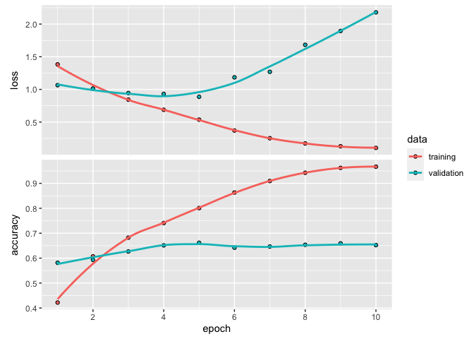
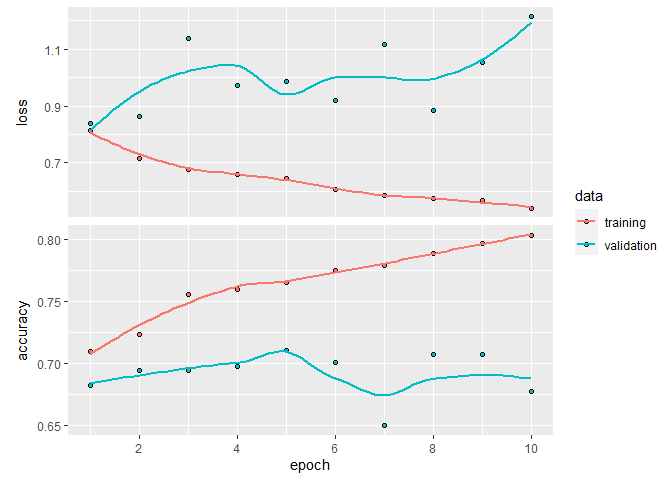
An important aspect to evaluate if your model was over- or underfitting, is to look at the evolution of the loss metric over the 30 epochs we’ve used :
plot(history)
`geom_smooth()` using formula 'y ~ x'
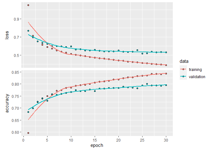
If this was the final step of your modelling, we could test the true quality of our model against the test set we had put aside earlier :
modele_keras %>%
  evaluate(x_test,y_test %>% to_categorical())
     loss  accuracy
0.5306777 0.7943122
As you can see from these numbers, our DL does a pretty good job. In fact, if you look at the Kaggle leaderboard for this challenge : https://www.kaggle.com/c/forest-cover-type-prediction/leaderboard such numbers would have put us in best couple of hundreds participants out of 1600. Keep in mind when looking at the leaderboard that some of these scores are probably not legitimate, as this challenge was based on publicly available data, which, sadly, also included the rows used by Kaggle to assess individual entries.
As you might have noticed, this first model rapidly overfits our data. You can see that in the loss function traces above, where at the fifth epoch, the model starts performing better with the training data than with the validation data. This is your number one sign of an overfitting model. In a balanced model, both curves should follow each other, converging onto their respecting final values. We could have probably squeezed a bit of performance by trying different model layouts (i.e. adding layers, changing the number of hidden nodes, etc), and some regularization techniques to combat overfitting, but that goes beyond the scope of this first example.
Also, some of you may have realized that this model is not better than the quick RF we built previously as a baseline. As stated before, classic models like RF perform really well at these kinds of tasks, so this phenomenon is not surprising at all.
How do computers see ?
Our first example above used what we could describe as simple, rectangular data, a format computers easily understand and process. Things get much more complicated when we talk about tasks like image recognition and classification. Our source material is also in a rectangular format (a picture is, after all, only a matrix of pixel values), but the techniques to understand what is inside the image are much more complicated.
It is true, you could train a RF model for image classification by feeding it a matrix of pixels as input. It might even work in some situations. But the problem with image classification is that, the target image is not necessarily exactly in the same place every time in the picture. It might also be a completely different color (imagine training your model on white cats and trying to detect a black cat), or a slightly different angle. Using each pixel in the image as a variable in a model can only get you so far.
This is where DL models really shine. They have a way to abstract features inside an image that generalizes much better than just looking at the individual pixel values, through a process callad convolution. DL models using convolution are usually called convolutional networks, or ConvNet for short.
ConvNets explained
Convolution layers are tools that extract local patterns inside images. They work as little moving windows (usually of 3x3 cells), called kernels, that filters a specific pattern across an image.
Each time the kernel is superposed to the image, the value of every cell from the kernel is multiplied by every corresponding cell in the image, and these values are then summed, to generate a new value in the resulting image.

Upon moving across all the original image, the resulting image contains information about the presence of a specific pattern, defined by the kernel. In ConvNet parlance, the resulting image from such a transformation is called a feature map …a map of all the features the kernel detected inside our original image.
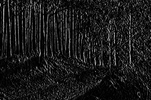
As an illustration, we can easily detect vertical edges in a image using the following kernel :
| -1 | 0 | 1 |
| -1 | 0 | 1 |
| -1 | 0 | 1 |
When we apply this kernel on the following image :
Linking to ImageMagick 6.9.12.3
Enabled features: cairo, fontconfig, freetype, heic, lcms, pango, raw, rsvg, webp
Disabled features: fftw, ghostscript, x11

We obtain a feature map of vertical edges :
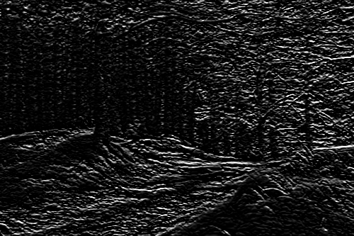
Conversely, if we apply this kernel :
| -1 | -1 | -1 |
| 0 | 0 | 0 |
| 1 | 1 | 1 |
We obtain a feature map of horizontal edges instead :
As a side note, many of the image enhancement features of photo editing software are simply kernels applied in just that way. For example, the famous pop effect is usually this defined by this kernel :
| 0 | -1 | 0 |
| -1 | 5 | -1 |
| 0 | -1 | 0 |
The exact kernels our ConvNet will use are not defined a priori, they are built from a randomized set of numbers, and optimized as any other parameter (i.e. weights) in our model.
A single convolutional layer may contain many such kernels, to detect all kinds of patterns inside the image. It builds a kind of vocabulary to describe the original image. The number of kernels in a layer is called the feature depth.
Things get even better when you stack a couple of these layers on top of one another. If you connect a second convolutional layer to the first one, this new layer will learn patterns about patterns, for example two diagonals connected together, or a diagonal crossed by a dot, etc. Upon connecting four or five layers this way, the ConvNet usually has enough freedom to describe just about any shape you could think of.
Please bear in mind that many details of the procedure are left for the reader to explore. For example, we won’t go into the details of how edges are managed with the moving window procedure, etc.
A hierarchy of features
In order for you ConvNet to work in the way described above and produce useful results, there is a general principle you need to follow when building your model.
The principle is that, as information moves along your ConvNet, the feature map needs to get deeper (i.e. you need to increase the number of kernels) and the size of the feature map (i.e. the number of pixels), needs to decrease. If you follow this recipe, your model should be able to create the hierarchy of information needed to solve your computer vision problem.
Increasing the depth of the feature map is pretty straightforward. For each layer you add, you change the filters parameter.
To reduce the size of the feature map as you get deeper in your stack of layers, the most common thing to do is to insert pooling layers between convolution layers. Usually, in computer vision models, one uses the max-pooling operation.
Max-pooling works a bit like a kernel, but instead of multiplying and then summing every cell, it just returns the maximum value inside its window. Also, instead of doing this by centering itself on every pixel from the image, the max-pooling operation does so in non-overlapping windows. A 2d max-pooling layer does effectively reduce the feature map size in half.

By Aphex34 - Own work;, CC BY-SA 4.0, Link
How does it predict anything?
If you’ve followed our model building steps up to this point, you might be wondering : how will such a model predict anything? And, in fact, we’ve omitted that part so far.
The way it will work is that, at the end of the stack of convolution/max-pooling layers, we’ll then attach what is called a flattening layer, which transforms our 3d tensor into a simpler, 1d structure, which we then feed to a dense layer and a final prediction layer, both of which will learn which of the ConvNet produced features correspond to each of our target classes.
An image classification example
OK, enough theory for now. Let’s code!
In order to try our hand at image classification, we’ll tackle as second Kaggle challenge : the flower recognition task : https://www.kaggle.com/alxmamaev/flowers-recognition
The dataset contains 4242 images from 5 flower species : daisy, dandelion, rose, sunflower and tulip. If you peek through the images, you’ll probably notice that this dataset is far from perfect. There are a couple of weird images, maybe even a couple of misclassifications… just like your are likely to find in a real world dataset.
Our goal is pretty simple : build a ConvNet, that will be capable of classifying a flower picture correctly in one of the five provided species.
Data preparation
When preparing such a dataset, the simplest way to organize your pictures is to have one folder per target category (here species). The Keras library offers us many functions that will handle the rest for us.
Note that the original dataset from the challenge has some strange issues, where inside one of the folder, you get again the five species folders with exactly the same pictures. I strongly suggest you download my cleaned-up folder instead : https://drive.google.com/drive/folders/16OxC0fZJ6nqkpxP2VxHyUYV8A-i5F0xb?usp=sharing
A dumb baseline
So, what would be a good baseline for our project? Surely, we cannot expect to dump all these pixels into a RF model and hope for the best. But, with 5 species and a relatively balanced dataset, a model predicting “dandelion” every time would still be right about 20% of the time.
So that will be our first target, to do best than our dumb dandelion model.
Configuration values
When attacking larger ML problem such as this one, it is a good idea to start off you script file with some configuration values :
dossier_images <- "data/flowers/complet/"
image_size <- 100
rescale <- 1/255
validation_split <- 0.2
seed <- 2551
batch_size <- 20
Everytime you realize you’re copy-pasting some number in your code, come back to this section and add the number there instead. That way, you’ll only need to change it in a single place and avoid yourself a lot of trouble.
I’ll define each of these numbers as we move along. The important thing for now is to notice that on my computer, the pictures are stored in a folder called “data/flowers/complet/”, but surely, in yours it will be a different place, so make sure you change this value right away.
Managing memory
One thing you’ll rapidly notice if you think about how your poor little laptop will handle our dataset, is that it’s probably not a good idea to load all these 4000+ images in memory at once. Your computer would just grind to a halt.
That’s why the Keras library offers us the (awkwardly named) data generators. The basic idea is that, instead of preparing a complete tensor ready to feed into the model like in your first example, we will, instead, build a function that Keras will to use when it needs more data to feed its model fitting process.
As of now, our function won’t generate data per se, but we’ll see later why its name says it is.
There are many function in Keras to build generators, but the one we will use here is called flow_images_from_directory, which, as its name implies load images from a directory. There also exists functions like flow_images_from_dataframe, where one of your column will contain the location of each image, etc.
train_generator <- flow_images_from_directory(
  directory = dossier_images,
  generator =  image_data_generator(rescale = rescale,validation_split = validation_split),
  target_size = c(image_size,image_size),
  batch_size = batch_size,
  seed = seed,
  subset = "training"
)
The first generator we build is the training-set generator. We point it to our image folder (directory). We then choose our generator function (image_data_generator) to which feed a rescaling factor.
You got to be careful here, because the terminology can get a little confusing. The rescale argument to image_data_generator is about scaling the values inside the image, and NOT about resizing the image.
We chose 1/255 because, as you might know, pixel values are stored in a 0-255 range, but tensor operations work much better on small numbers. We also inform this generator that the size of the validation split will be 20% (i.e. 0.2).
Then, back to the arguments for flow_images_from_directory, we ask it to resize our images (100 x100 px) to reduce our memory footprint. We then set the batch_size argument to 20, which asks Keras to only load 20 images into memory at once. Finally, we specify a seed for the random generator to get consistent train/validation splits between runs, and ask that this particular function returns the training part of our dataset.
We then create a second generator, with exactly the same arguments, except for the subset, which we set to validation instead of training.
validation_generator <- flow_images_from_directory(
  directory = dossier_images,
  generator =  image_data_generator(rescale = rescale,validation_split = validation_split),
  target_size = c(image_size,image_size),
  batch_size = batch_size,
  subset = "validation"
)
As you might have guessed, it would have also been a reasonable strategy to manually separate our images ourselves into a training and a validation folder, and point our two generators there instead of using the subsets arguments, but I find this strategy much less hassle.
Your first ConvNet
So, the time has finally come to write our ConvNet model. As we explained above, the ConvNet part of our model is a series of convolution layers, alternating with max-pooling layers, so that, as the depth of the feature map increases (number of filters), the size of the map itself is reduced.
At the end of the ConvNet, we connect a flatten layer to transform our feature map into a 1d tensor, which we feed into a densely connected layer and a classification layer.
Notice that here, our last layer has 5 units, because we have 5 flower species to identify.
model <- keras_model_sequential() %>%

  # ConvNet
  layer_conv_2d(filters = 32,kernel_size = c(3,3),activation = "relu",
                input_shape = c(image_size,image_size,3)) %>%
  layer_max_pooling_2d(pool_size = c(2,2)) %>%
  layer_conv_2d(filters = 64,kernel_size = c(3,3),activation = "relu") %>%
  layer_max_pooling_2d(pool_size = c(2,2)) %>%
  layer_conv_2d(filters = 128,kernel_size = c(3,3),activation = "relu") %>%
  layer_max_pooling_2d(pool_size = c(2,2)) %>%
  # Flatten and classify
  layer_flatten() %>%
  layer_dense(units = 512, activation = "relu") %>%
  layer_dense(units = 5, activation = "softmax")
If you want to have an overview of the kind of beast you are working with now, you can type your model name in the console, and see that…
model
Model
Model: "sequential"
________________________________________________________________________________
Layer (type)                        Output Shape                    Param #
================================================================================
conv2d_2 (Conv2D)                   (None, 98, 98, 32)              896
________________________________________________________________________________
max_pooling2d_2 (MaxPooling2D)      (None, 49, 49, 32)              0
________________________________________________________________________________
conv2d_1 (Conv2D)                   (None, 47, 47, 64)              18496
________________________________________________________________________________
max_pooling2d_1 (MaxPooling2D)      (None, 23, 23, 64)              0
________________________________________________________________________________
conv2d (Conv2D)                     (None, 21, 21, 128)             73856
________________________________________________________________________________
max_pooling2d (MaxPooling2D)        (None, 10, 10, 128)             0
________________________________________________________________________________
flatten (Flatten)                   (None, 12800)                   0
________________________________________________________________________________
dense_1 (Dense)                     (None, 512)                     6554112
________________________________________________________________________________
dense (Dense)                       (None, 5)                       2565
================================================================================
Total params: 6,649,925
Trainable params: 6,649,925
Non-trainable params: 0
________________________________________________________________________________
your model will need to train 6+ million parameters… which is just what you might expect for this kind of task!
We can now compile our model, with the same code as before :
model %>% compile(
  optimizer = "rmsprop",
  loss = "categorical_crossentropy",
  metrics = c("accuracy")
)
And finally, launch the model fitting, which might take a couple of minutes to run :
history <- model %>%
  fit(
    x = train_generator,
    epochs = 10,
    steps_per_epoch = round(train_generator$n / batch_size),
    validation_data = validation_generator,
    validation_steps = round(validation_generator$n / batch_size)
  )
You’ll see that here, although some arguments look a lot like they did before, they are subtly different. Both x and validation are now function names instead of actual matrices.
You’ll also notice that we are now required to define how many steps (i.e. batches), we want our model to take in each epoch. For now, we simply divide the total number of images by the size of a batch. This information is needed because, as we’ll see later, data generators are not limited by our original images and could create some on the fly.
So, how did our first model do?
plot(history)
`geom_smooth()` using formula 'y ~ x'
history
Final epoch (plot to see history):
        loss: 0.105
    accuracy: 0.9669
    val_loss: 2.179
val_accuracy: 0.6523
So, there are many good news here. First of all, our validation accuracy is at 65%. In our context, it is a very good result. Remember that a dumb, dandelion model would be right only 20% of the time.
The other good news is that, our model quickly over-adjusted to our training data. At epoch 3, training loss is already better than the validation. This means that our model is probably complex enough for the task at hand. We can now try some regularization techniques.
If at that point, our model was not overfitting, our next steps would involve playing with our ConvNet layers, probably adding some. Doing so, it will be important to think about the amount of information left after each layer. Here, starting with a 100 x 100 px image, our last max-pooling layers ends with a feature map of dimensions 10x10, which is decent. If you had added another layer to our ConvNet, our last feature map would have probably been too small to convey any meaningful information. In order to add more layers, we would have also needed to work with bigger images, which means a slower training process, etc.
Advanced techniques
Fighting overfitting
Fighting the overfitting tendency of your model is something you will face every time you attack a DL problem.
Many techniques have been devised for this purpose, including regularizing the weights in your network, either with L1 or L2 norms (think Lasso and Ridge regression).
One must also think about reducing the size of the model per se. Maybe having fewer layers or fewer hidden units per layer might help. Sadly, there is no precise recipe for that, only experience can help you figuring out the appropriate network size for a given problem.
For ConvNets, there are two additional techniques that are often used. Adding dropout and data augmentation. Both of which we will try below.
Adding dropout
If I had asked you to come up with a way to reduce overfitting in a ML model, I’m pretty sure very few of you would have suggested : Hey Charles, how about: every time we treat an input with the model, we randomly drop half the coefficients to zero?
But it is, believe it or not, one of the best anti-overfitting measure in DL models. It is said that the inventor of the method got his idea while thinking about bank tellers, which kept getting shuffled or moved around, and as a result, he almost never talked to the same individual. He realized at that point that such a process was key to preventing frauds, as each teller was always working with new co-workers. The same phenomenon applies to nodes in our network. By randomly zeroing a fraction of them for each input, we keep coefficients independent of one another, and prevent them from learning unimportant patterns while their neighbour does the job.
Of course, at testing time, there are no dropout values in the model, but an equivalent scaling must be applied to the outputs, because now we have all the weights coming-in instead of only a fraction (Don’t worry, you don’t have to manage that scaling manually).
In practice, in a ConvNet, you only apply dropout at the classification part of your model, not within the convolutional section.
So, let’s see how it goes by adding two dropout layers at classification part of our model. Our code is exactly the same as above, except for the dropout layer above and below the dense layer
model_do <- keras_model_sequential() %>%
  layer_conv_2d(filters = 32,kernel_size = c(3,3),activation = "relu",input_shape = c(image_size,image_size,3)) %>%
  layer_max_pooling_2d(pool_size = c(2,2)) %>%
  layer_conv_2d(filters = 64,kernel_size = c(3,3),activation = "relu") %>%
  layer_max_pooling_2d(pool_size = c(2,2)) %>%
  layer_conv_2d(filters = 128,kernel_size = c(3,3),activation = "relu") %>%
  layer_max_pooling_2d(pool_size = c(2,2)) %>%
  layer_flatten() %>%
  layer_dropout(rate = 0.5) %>%
  layer_dense(units = 512, activation = "relu") %>%
  layer_dropout(rate = 0.5) %>%
  layer_dense(units = 5, activation = "softmax")

model_do %>% compile(
  optimizer = "rmsprop",
  loss = "categorical_crossentropy",
  metrics = c("accuracy")
)

history_do <- model_do %>%
  fit(
    x = train_generator,
    epochs = 10,
    steps_per_epoch = round(train_generator$n / batch_size),
    validation_data = validation_generator,
    validation_steps = round(validation_generator$n / batch_size)
  )

plot(history_do)
`geom_smooth()` using formula 'y ~ x'
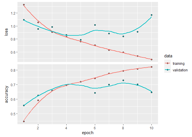
history_do
Final epoch (plot to see history):
        loss: 0.4885
    accuracy: 0.821
    val_loss: 1.17
val_accuracy: 0.6477
So, that is not much better than our initial model, although the validation errors are a bit unstable between epochs, which could be due to the small nature of our dataset.
As you’ll soon learn, the fine tuning part of DL modelling can be many long hours for very little return, and it is more an art than a science.
Data augmentation
Another strategy one can use to reduce overfitting in a ConvNet is to apply data augmentation techniques. This technique does exactly as the name implies : it creates data for you. Of course, not totally random data. Just random enough do help your model generalize from the data you gathered.
The basic idea is to let your data generator play with your images, to rotate them, flip them, crop them, etc.
For example, one of our daisy could end up in any of these configurations in every epoch of our model training process :
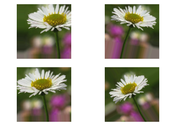
When employing such techniques, it is important to think about what kind of transformation would make sense for our data, and which would not. For example, for car pictures, vertical flips would not make much sense, but horizontal flips would be a great idea. On the other hand, to analyze electrocardiograms, horizontal flips would be a very bad idea, as the left to right sequence is associated with the time domain, etc.
There are tens of options to choose from when building a data augmentation generator. For the problem at hand, I choose 3 options, which are rotation, shear and horizontal flip :
aug_train_generator <- flow_images_from_directory(
  directory = dossier_images,
  generator =  image_data_generator(

    # Data augmentation
    rotation_range = 40,
    shear_range = 0.2,
    horizontal_flip = TRUE,

    # Other arguments, as used above...
    rescale = rescale,
    validation_split = validation_split
  ),
  target_size = c(image_size,image_size),
  batch_size = batch_size,
  seed = seed,
  subset = "training"
)
So, now, let’s try this new augmented data generator with our flowers model. Note that I needed to add the reset_states command before fitting our model again. If we did not do that, the fitting process would resume from where it stopped the last time (which might be useful to do in some circumstances, but it’s not what were aiming for here).
history_aug <- model %>%
  reset_states %>%
  fit(
    x = aug_train_generator,
    epochs = 10,
    steps_per_epoch = round(aug_train_generator$n / batch_size),
    validation_data = validation_generator,
    validation_steps = round(validation_generator$n / batch_size)
  )

plot(history_aug)
`geom_smooth()` using formula 'y ~ x'
history_aug
Final epoch (plot to see history):
        loss: 0.5412
    accuracy: 0.8033
    val_loss: 1.213
val_accuracy: 0.6779
So, that is a bit better than our initial model, but not by much.
You might also be tempted to combine both dropout and augmentation in a single model and I encourage you to give it a try, although in most cases, the model will rarely improve by combining both techniques.
Pretrained ConvNets
A last technique we might try to improve our model, especially on small datasets, such as our flowers identification problem is to use a pretrained ConvNet. As we’ve talked about, the ConvNet part of our model is building a vocabulary to describe our images. It learns to define edges, shapes, etc.
The important thing is that, the vocabulary building part of the learning process need not to happen necessarily on our dataset. The feature extraction could be much powerful and robust if it was trained on million of images instead of the few thousands we have here.
That is why Keras comes with a bunch a pre-packaged ConvNets, ready to use.
To run our little example today, we’ll use the VGG16, which was trained on the ImageNet database, which has more 14 million of images to categorize into over 1000 categories. The VGG16 architecture achieved a 92.7 % accuracy on that difficult task (https://neurohive.io/en/popular-networks/vgg16/).
We’ll initialize our base layer with the following code :
conv_base <- application_vgg16(
  weights = "imagenet",
  include_top = FALSE,
  input_shape = c(image_size, image_size, 3)
)
Notice that we need first to mention that we don’t want the top of the model (the classification part), which we want tailored to our specific problem. Also we need to mention the shape of our input tensor, as it is not necessarily the same as the one used to train the pretrained network.
pt_model <- keras_model_sequential() %>%
  conv_base %>%
  layer_flatten() %>%
  layer_dense(units = 256, activation = "relu") %>%
  layer_dense(units = 5, activation = "softmax")
One last important thing to do before compiling and fitting this model is to freeze our shiny new base we’ve activated. We don’t want our fitting process to start changing these pretrained weights around.
freeze_weights(conv_base)
Now we are ready to compile and run our model. You’ll notice that this model runs much slower than the previous. We a probably reaching the limit of what can be reasonably run on your personnal laptop…
You’ll also notice that here, we need to change the learning rate value of our rmsprop optimizer (the lr argument). Usually, the default values for the optimizer are reasonably decent and will get you some pretty good results. Here however, as we’re working with a partially frozen ConvNet, we need to consequently adjust the learning rate manually to a slower value.
pt_model %>% compile(
  loss = "categorical_crossentropy",
  optimizer = optimizer_rmsprop(lr = 2e-5),
  metrics = c("accuracy")
)

pt_history <- pt_model %>% fit_generator(
  aug_train_generator,
  steps_per_epoch = round(aug_train_generator$n / batch_size),
  epochs = 10,
  validation_data = validation_generator,
  validation_steps = round(validation_generator$n / batch_size)
)
Warning in fit_generator(., aug_train_generator, steps_per_epoch =
round(aug_train_generator$n/batch_size), : `fit_generator` is deprecated. Use `fit`
instead, it now accept generators.
plot(pt_history)
`geom_smooth()` using formula 'y ~ x'
pt_history
Final epoch (plot to see history):
        loss: 0.6883
    accuracy: 0.756
    val_loss: 0.7133
val_accuracy: 0.7523
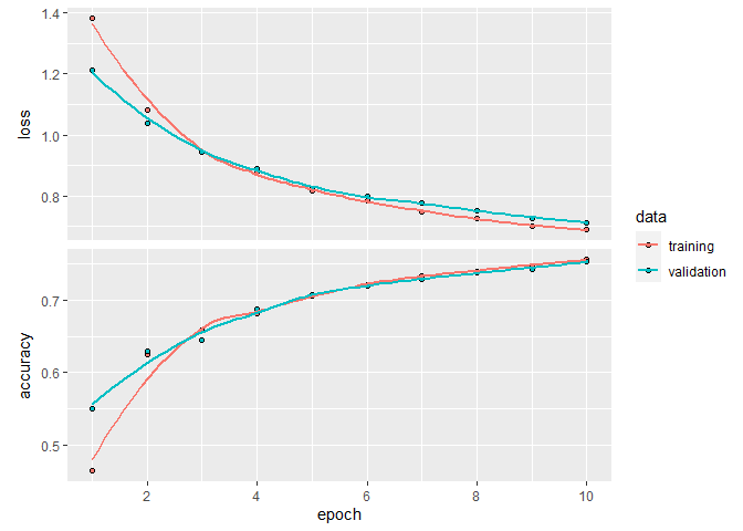
So again, that is a bit better than our previous attempts. With a bit of additional tuning, more epochs, more pixels per image etc., it should be possible to achieve at least 90 % accuracy with our model, but I’ll leave it to you to try it out.
GPU acceleration
As you see, in DL problems, we rapidly hit hardware limitations when running code on our laptop’s CPU.
The good news is that Keras is able to take advantage of hardware acceleration : i.e. it can run code on a graphic card (GPU) much faster, just like your games would do.
But not on any GPU. You GPU needs to come NVidia, and be CUDA-enabled. You can find a list of CUDA-enabled graphic cards here : https://developer.nvidia.com/cuda-gpus.
The process to activate Keras’ GPU support is a bit involved and goes beyond what we have time to do in this workshop. You need to install at least two additional pieces of software (the CUDA framework, as well as cuDNN). Once this is done, you then need to install the hardware accelerated version of Keras with :
install_keras(tensorflow = "gpu")
Hopefully, once all these steps are completed, the remainder of the code just runs as-is, without any changes. That’s the magic of Tensorflow!
Typical workflow
To recap everything we’ve said above, here’s how your typical DL project should go :
- Define your problem. What are your inputs? What are the expected outputs?
- Choose how you’ll measure success (RMSE, accuracy, etc.)
- Decide how you’ll evaluate your model (separate training and test set, cross-validation, etc?)
Here a quick recap of the usual activation and loss functions used for classic machine learning problems.
| Problem type | Activation function | Loss function |
|---|---|---|
| Binary classification | sigmoid | binary_crossentropy |
| Multiclass classification | softmax | categorical_crossentropy |
| Regression 0-1 values | sigmoid | mse or binary_crossentropy |
| Regression (other) | (none) | mse |
- Build a first model that does better than a basic baseline.
- Improve that model so that it can overfit (adding layers, growing layers, adding more epochs).
- Regularize that model (dropouts, etc.) and tune its hyperparameters (dropout rate, number of hidden layer, number of hidden units, learning rate, etc.).
Of course, we have barely scratched the surface of what’s possible with DL models. Nowadays, these models are also used in time series analysis, sound identification, video analysis, etc.
There are also many artistic endeavours using these kind of models, for example in story writing (https://www.thedrum.com/opinion/2019/01/22/neural-storytelling-how-ai-attempting-content-creation) and visual arts (https://www.kdnuggets.com/2015/09/deep-learning-art-style.html).
So, go out there, get some data and get coding! Who knows where next breakthrough will come from!
References
Most of this workshop is based on the book Deep Learning with R (2018) from Keras’ author François Chollet and RStudio founder J.J. Allaire. It is clearly your best starting point to get started with DL with R.
Both learning problems shown here came from Kaggle.com. Kaggle is an excellent source of ML problems if you want to cut your teeth on some real life problems and see how your solution compares to other attempts. If you take a look a the proposed solutions for any challenge, you’ll quickly realize that Python is currently the lingua franca of DL. If you main interest lies more in DL than in statistical inference and modelling as we usually do in ecology, I strongly encourage you to learn Python.
As usual, RStudio has an excellent cheat sheet which summarizes every possible layer type, as well a many operations we have not covered here (e.g. saving and loading a model, etc.)
Finally, for in depth info and the latest developments, you can take a look at Keras’ official website at https://keras.io/