Introduction to Machine Learning

Charles Martin

May 2019

• Introduction
  • Necessary packages and functions
  • Faces dataset
  • Non-faces dataset
  • How to enter such images inside a statistical model
  • Extracting features from the faces dataset
  • Extracting features from the non-faces dataset
  • Preparing the complete dataset
  • Splitting the complete dataset
• Model training
  • Support-Vector Machine
  • Adjusting SVM hyperparameters using cross-validation
  • Training a model with the optimal hyperparameters values
  • Checking model performance
• Searching for faces in a new image
  • Visualising the results
• Problems and solutions
  • Multiple detection
  • False-positives overload
  • Size differences

Introduction

Today well run through a simple example of machine learning with R, by traning a model to find faces inside an image.

Necessary packages and functions

library(tidyverse) # data manipulation
library(magick) # image manipulation
library(e1071) # svm model
library(OpenImageR) # HOG
source("Algorithmes.R") # Non-max suppression + bug HOG

Faces dataset

There is no secret here, one has to look at the original image, spot faces and note their coordinates. I used ImageJ to accelerate this process.

Here’s a preview of the coordinates file :

coords <- read_tsv(
  "images/page1/full.txt",
  col_names = c("X","Y")
)

head(coords)

# A tibble: 6 x 2
      X     Y
  <dbl> <dbl>
1  476.  93.7
2  511. 342  
3  608. 524.
4  541  553.
5  521  570.
6  486  566  

For this workshop, I noted 90 faces. In a real world application, you’d need many times that number to get acceptable results.

Then, using the magick package, we’ll extract a thumbnail for each of these faces :

full <- image_read("images/page1/full.jpg")
thumb_size <- 16

for (i in 1:nrow(coords)) {
  full %>%
    image_crop(
      geometry_area(
        thumb_size,
        thumb_size,
        coords[[i,"X"]] - thumb_size/2, # Je sais que j'ai cliqué au milieu du visage...
        coords[[i,"Y"]] - thumb_size/2
      )
    ) %>%
    image_write(paste0("images/page1/faces/",i,".jpg"))
}

Non-faces dataset

For this dataset, we’ll simple pick random locations inside the original image. In real life situations, you’d need to inspect each thumbnail to make sure that they are not in fact faces.

for (i in 1:600) {

  random_x <- sample(
    1:(image_info(full)$width - thumb_size),
    1
  )
  random_y <- sample(
    1:(image_info(full)$height - thumb_size),
    1
  )

  full %>%
    image_crop(
      geometry_area(
        thumb_size,
        thumb_size,
        random_x,
        random_y
    )
  ) %>%
  image_write(paste0("images/page1/nonfaces/",i,".jpg"))

}

How to enter such images inside a statistical model

We’ll apply the Histogram of Oriented Gradients method, which will generate us a series of features that can be used as variables in our models.

Extracting features from the faces dataset

files <- dir("images/page1/faces", full.names = TRUE)
faces <- HOG_apply2(files)

Extracting features from the non-faces dataset

files <- dir("images/page1/nonfaces", full.names = TRUE)
nonfaces <- HOG_apply2(files)

Preparing the complete dataset

X <- rbind(
  faces,
  nonfaces
)

Y <- as_factor(
  rep(c("face","nonface"),
    c(nrow(faces),nrow(nonfaces))
  )
)

Splitting the complete dataset

In machine learning, one typically create a neat seperation between data used for model training and data used for model testing. Here, will keep 75% of the dataset for hyperparameter optimisation and 25% to test the final model.

sample <- sample.int(
  n = nrow(X),
  size = floor(.75*nrow(X))
)

X_train <- X[sample, ]
X_test  <- X[-sample, ]

Y_train <- Y[sample]
Y_test  <- Y[-sample]

Model training

Support-Vector Machine

Now, we need a mathematical model that will make predictions about our label of interest (face or non-face) from the information contained in our images ( encoded as histogram of gradient features). One could easily used simple (kNN) or more classic (logistic regressions), but today we’ll try Support-Vector Machines.

Adjusting SVM hyperparameters using cross-validation

tuned_params <- tune.svm(
  x = X_train,
  y = Y_train,

  gamma = c(0.0001,0.001,0.01),
  cost = c(1,10,100),
  tunecontrol = tune.control(cross = 4)

)

tuned_params

Parameter tuning of 'svm':

- sampling method: 4-fold cross validation

- best parameters:
 gamma cost
 0.001   10

- best performance: 0.07161598

Training a model with the optimal hyperparameters values

trained_model <- svm(
  x = X_train,
  y = Y_train,
  gamma = tuned_params$best.parameters$gamma,
  cost = tuned_params$best.parameters$cost,
  probability = TRUE
)

Checking model performance

pred <- predict(trained_model, X_test)
res <- table(pred, Y_test)
res

         Y_test
pred      face nonface
  face      17       4
  nonface    6     146

There are many ways to test for the quality of a model predicting labels such as the one above.

Accuracy : (TP + TN) / Total

Proportion of correct classifications. Equivalent to the classic R2 metric in regression.

May be problematic if the studied phenomenon is very rare or very common.

Precision : TP / (TP + FP)

Proportion of detections that are correct. Especially useful if false negative are important to this problem.

Recall : TP / (TP + FN)

Can be thought of as the model’s detection probability. Useful if you want to make that you don’t miss any cases.

# Accuracy
sum(diag(res)) / sum(res)

[1] 0.9421965

# Precision
res[1,1] / (res[1,1] + res[1,2])

[1] 0.8095238

# Recall
res[1,1] / (res[1,1] + res[2,1])

[1] 0.7391304

Searching for faces in a new image

We first need to determine with which precision we want to explore the image. Here, I selected to slide my search window over every other pixel.

search_area <- image_read("images/page2/search_area.jpg")

seq_x <- seq(
  from = 1,
  to = image_info(search_area)$width - thumb_size,
  by = 2
)
seq_y <- seq(
  from = 1,
  to = image_info(search_area)$height - thumb_size,
  by = 2
)

And the face search per-se :

  face_coords <- tibble(
  x = NA,
  y = NA,
  probability = NA
  )

  for (x in seq_x) {
  for (y in seq_y) {

    thumb <- image_crop(
      search_area,
      geometry_area(
        thumb_size,
        thumb_size,
        x,
        y)
    )

    h <- HOG(
      as.integer(image_data(thumb))/255,
      cells = 8,
      orientations = 8
    )

    p <- predict(trained_model,t(h), probability = TRUE)
    if (p == "face") {
      face_coords <- face_coords %>%
        add_row(
          x = x,
          y = y,
          probability = attr(p,"probabilities")[2]
        )
    }
  }
  }

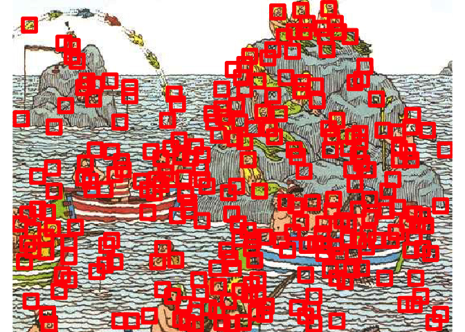
Visualising the results

image_ggplot(search_area) +
  geom_rect(
    data = face_coords,
    aes(
      xmin = x,
      xmax = x + thumb_size,
      ymin = y,
      ymax = y + thumb_size
    ),
    fill = NA,
    color = "red",
    size = 2
  )

Warning: Removed 1 rows containing missing values (geom_rect).

Problems and solutions

Multiple detection

Since our algorithm is fairly robust (which is what we want to achieve), the same face was detected many times.

One classic way to the with this is the Non-max Suppression algorithm.

filtered_faces <- non_max_suppression(face_coords)

image_ggplot(search_area) +
  geom_rect(
    data = filtered_faces,
    aes(
      xmin = x,
      xmax = x + thumb_size,
      ymin = y,
      ymax = y + thumb_size
    ),
    fill = NA,
    color = "red",
    size = 2
  )

False-positives overload

So far, our algorithm detects many things that aren’t faces in the new image. Machine Learning need a lot of examples of non-faces, much more than a human would need to understand the problem.

One way around this issue is to save every false positive the algorithm detects in a folder, and combine it with the original non-faces dataset when traning the model.

Size differences

As of now, our algorithm searches only at a single scale. In real life, we should probably search the image at many different scales