PARAFAC part 1 - Data conditioning and indices
Jade Dormoy-Boulanger and Mathieu Michaud
May 2022
- Before starting
- Import raw data from staRdom package
- Check data
- Data preparation and correction
- Choosing fluorescence peaks and indices
- Absorbance indices
PARAFAC analysis and absorbance and fluorescence indices are statistical analyses used to characterize dissolved organic matter (DOM). They provide informations on the DOM composition, source and molecular form. These methods use emission and excitation matrices obtained by a fluorescence spectrophotometer. Usually these statistical analyses are performed on the Matlab software, but the staRdom package from R also allows to perform these analyses.
This is an adaptation from a tutorial from Matthias Pucher, who is the staRdom developper, called “PARAFAC analysis of EEM data to separate DOM components in R”. We will use the example datasets contained within the staRdom package for this tutorial, but we also tried the method with real data as well, and we confident about the efficiency of the codes.
Link for Matthias Pucher tutorial: https://cran.r-project.org/web/packages/staRdom/vignettes/PARAFAC_analysis_of_EEM.html
The R method for PARAFAC and fluorescence indices is equvalent to the Matlab method, as this paper from Pucher et al. (2019) demonstrate it: https://doi.org/10.3390/w11112366
Part 1: Introduction to absorbance indices
PARAFAC analysis are usually performed along fluorescence and absorbance indices. As these analysis requiered a lot of time to run and are quite heavy to understand, we have separated indices from PARAFAC. We will start with this indices, since the required data conditionning is the same as for the PARAFAC analysis. We will then be able to use our emmission and excitation matrices (EEMs) from the indices to perform the PARAFAC.
Before starting
The first step is to install and load the staRdom and to check how many cores your computer have. The best calculation speed is acheived by setting the number of cores within somme of the most demanding function that we will be using. We will also need the following packages: dplyr, tidyr and eemR (eemR is installed with the staRdom package installation).
#packages loading
library(staRdom)
library(dplyr)
library(tidyr)
library(eemR)
#speed calculation optimization
cores <-detectCores(logical = FALSE) # how many cores
cores # I have 4 cores
## [1] 4
Import raw data from staRdom package
We will use the example data that comes with the staRdom package. If you are using your own data, here’s some advices:
- EEMs and absorbance files name should be identical
- Files name should not contain “-“ nor starting with a number
- Files need to be in csv format with commas separator (no semicolons!)
- EEMs folders should also contain your blanks and their name have to have one of these terms: “nano”, “miliq”, “milliq”, “mq” ou “blank”
- Use directly absorbance_read() and eem_read() with your computer path to your data as argument (ex: eem_list <- eem_read(“C:/Users/Bureau/Doctorat /Donnees/PhD/DonneesR/PARAFAC-2020-brute/EEM”, recursive = T, import_function = “cary”)
- For eem_read(), you can set your spectrofluorometer brand with the argument import_function. staRdom actually support Varian Cary Eclipse (“cary”), Horiba Aqualog (“aqualog”), Horiba Fluoromax-4 (“fluoromax4”), Shimadzu (“shimadzu”), Hitachi F-7000 (eem_hitachi) and generic csv files (eem_csv)
system.file()
## [1] "C:/PROGRA~1/R/R-41~1.1/library/base"
#Absorbance
raw_abs<- system.file("extdata/absorbance", package = "staRdom")#data path
absorbance <- absorbance_read(raw_abs, cores = cores)#the data,will convert all the files to one dataset
#EEMs
eem<-system.file("extdata/EEMs", package = "staRdom")#path
eem_list <- eem_read(eem, recursive = TRUE, import_function = eem_csv) #the data, will convert to a list object
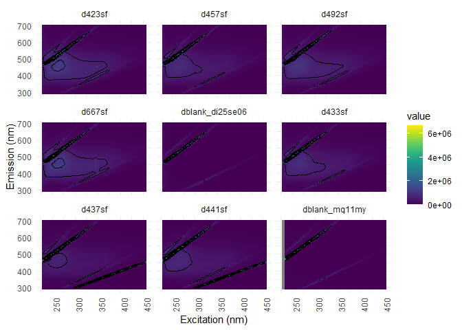
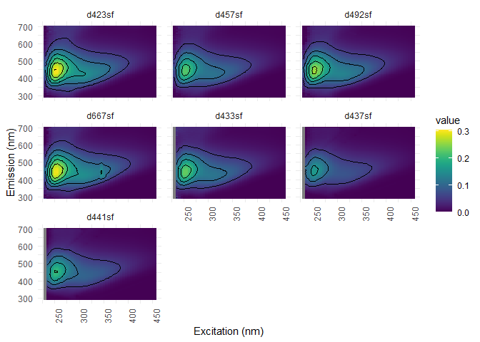
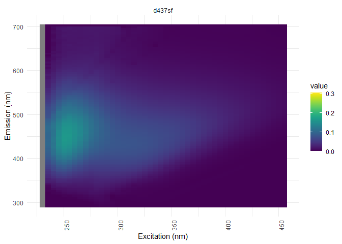
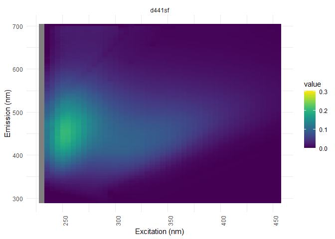
eem_overview_plot(eem_list, spp=9, contour = TRUE)
## [[1]]
## Warning: Removed 104 rows containing non-finite values (stat_contour).
#Metadata
metatable <- system.file("extdata/metatable_dreem.csv",package = "staRdom") #path
meta <- read.table(metatable, header = TRUE, sep = ",", dec = ".", row.names = 1) # les métadonnées

#If you are using your own data, you can create your metadat with the following code
eem_metatemplate(eem_list, absorbance) %>%
  write.csv(file="metatable.csv", row.names = FALSE)
Check data
The data check can be performed using eem_checkdata():
- NAs (NAs_in_EEMs)
- wavelength range mismatches (between EEMs: EEMs_more_data_than_smallest ; absorbance vs EEMs: EEM_absorbance_wavelength_range_mismatch)
- Incomplete data (EEMs without absorbance: EEMs_missing_absorbance; Absorbance without EEMs: Absorbance_missing_EEMs; EEMs without metadata: EEMs_missing_metadata; metadata without EEMs: Metadata_missing_EEMs)
- inconsistencies (duplicates, invalid)in samples names between EEM, absorbance and metadata (Duplicate_EEM_names, Duplicate_absorbance_names, invalid_EEM_names, invalid_absorbance_names,Duplicates_metatable_names)
- No correction applied to the data (missing_data_correction)
Analysis can tolerate up to 15%-20% of NAs. Above that, interpolation is strongly advised.
problem <- eem_checkdata(eem_list,absorbance,meta,metacolumns = c("dilution"),error=FALSE)
## NAs were found in the following samples (ratio):
## d423sf (0), d457sf (0), d492sf (0), d667sf (0), dblank_di25se06 (0), d433sf (0), d437sf (0), d441sf (0), dblank_mq11my (0.02),
## Please consider interpolating the data. It is highly recommended, due to more stable and meaningful PARAFAC models!
## EEM samples missing absorbance data:
## dblank_di25se06 in
## C:/Users/martich/Documents/R/win-library/4.1/staRdom/extdata/EEMs/di25se06
## dblank_mq11my in
## C:/Users/martich/Documents/R/win-library/4.1/staRdom/extdata/EEMs/mq11my
problem
## $Possible_problem_found
## [1] TRUE
##
## $NAs_in_EEMs
##          d423sf          d457sf          d492sf          d667sf dblank_di25se06
##      0.00000000      0.00000000      0.00000000      0.00000000      0.00000000
##          d433sf          d437sf          d441sf   dblank_mq11my
##      0.00000000      0.00000000      0.00000000      0.02173913
##
## $EEMs_more_data_than_smallest
## character(0)
##
## $missing_data_correction
## [1] NA
##
## $EEMs_missing_absorbance
## [1] "dblank_di25se06" "dblank_mq11my"
##
## $Absorbance_missing_EEMs
## character(0)
##
## $Duplicate_EEM_names
## character(0)
##
## $Duplicate_absorbance_names
## character(0)
##
## $invalid_EEM_names
## character(0)
##
## $invalid_absorbance_names
## character(0)
##
## $EEM_absorbance_wavelength_range_mismatch
## NULL
##
## $Duplicates_metatable_names
## character(0)
##
## $EEMs_missing_metadata
## NULL
##
## $Metadata_missing_EEMs
## NULL
Data preparation and correction
Here, we’ll discuss several important corrections for performing the analysis behind trustable indices and PARAFAC results.
Samples name
eem_name_replace() allows to change files name within your EEM list object. For the staRdom data, we want to eliminate “(FD3)”, which originates from the spectrofluorometer conversion to txt files. Also, the absorbance data files don’t have this in their files names (remember, we want identical files names for both absorbance and EEMs!!!)
eem_list <- eem_name_replace(eem_list,c("\\(FD3\\)"),c(""))
Absorbance baseline correction
Usually the absorbance correction is between 680 and 700 nm.
absorbance <- abs_blcor(absorbance,wlrange = c(680,700))
Spectral correction
Spectral correction eliminate the instrument specific influence on EEMs. Usually instruments will provide, along the data, two correction files (one for excitation and one for emission). If you are using your own data, you can set the data.table::fread() argument to your data path (ex: data.table::fread(“C:/Bureau/Doctorat/Donnees/PhD/DonneesR/PARAFAC_Numerilab/CorrFiles/Ex_Corr.csv”)).
# Excitation
excorfile <- system.file("extdata/CorrectionFiles/xc06se06n.csv",package="staRdom")# path
Excor <- data.table::fread(excorfile)#data

#Emission
emcorfile <- system.file("extdata/CorrectionFiles/mcorrs_4nm.csv",package="staRdom")#path
Emcor <- data.table::fread(emcorfile)#data

#Ajust EEMs range to cover vector corrections
eem_list <- eem_range(eem_list,ex = range(Excor[,1]), em = range(Emcor[,1]))#create spectral range
eem_list <- eem_spectral_cor(eem_list,Excor,Emcor)#correction
Blank substraction
Blanks must have in their files name “nano”, “miliq”, “milliq”, “mq” or “blank”. They are useful for the Raman correction and will be substracted from every sample to reduce systematic erreors and scattering. If several blanks are used, they will be averaged.
# extending and interpolation data
eem_list <- eem_extend2largest(eem_list, interpolation = 1, extend = FALSE, cores = cores)

# blank substraction
eem_list <- eem_remove_blank(eem_list)
## A total of 1 blank EEMs will be averaged.
## A total of 1 blank EEMs will be averaged.
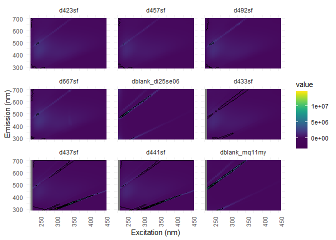
eem_overview_plot(eem_list, spp=9, contour = TRUE)
## [[1]]
## Warning: Removed 416 rows containing non-finite values (stat_contour).

Inner-filter effect (IFE) correction
IFE appears when excitation light is absorbed by chromophores (colored particules). The IFE correction method for EEMs uses absorbance data.
eem_list <- eem_ife_correction(eem_list,absorbance, cuvl = 5)#culv = cuvette length (cm)
## d423sf
## Range of IFE correction factors: 1.0004 1.0288
## Range of total absorbance (Atotal) : 1e-04 0.0049
##
## d457sf
## Range of IFE correction factors: 1.0003 1.0208
## Range of total absorbance (Atotal) : 1e-04 0.0036
##
## d492sf
## Range of IFE correction factors: 1.0004 1.0241
## Range of total absorbance (Atotal) : 1e-04 0.0041
##
## d667sf
## Range of IFE correction factors: 1.0004 1.0249
## Range of total absorbance (Atotal) : 1e-04 0.0043
## Warning in FUN(X[[i]], ...): No absorbance data was found for sample
## dblank_di25se06!No absorption data was found for sample dblank_di25se06!
## d433sf
## Range of IFE correction factors: 1.0003 1.0241
## Range of total absorbance (Atotal) : 1e-04 0.0041
##
## d437sf
## Range of IFE correction factors: 1.0002 1.0131
## Range of total absorbance (Atotal) : 0 0.0023
##
## d441sf
## Range of IFE correction factors: 1.0002 1.016
## Range of total absorbance (Atotal) : 0 0.0028
## Warning in FUN(X[[i]], ...): No absorbance data was found for sample
## dblank_mq11my!No absorption data was found for sample dblank_mq11my!
#it's normal that there is no absorbance data for the blanks...they will be removed later

eem_overview_plot(eem_list, spp=9, contour = TRUE)
## [[1]]
## Warning: Removed 416 rows containing non-finite values (stat_contour).
Raman normalization
Fluorescence intensity can change between instruments, parameters and days of analysis. Therefore, it needs to be normalized on a standard scale of Raman units by dividing all intensities by the area of the Raman’s peak (excitation at 350nm within emission between 371nm and 428nm) of an ultrapure water sample. Here we will use the ultrapure blanks.
eem_list <- eem_raman_normalisation2(eem_list, blank = "blank")
#Raman correction, blank = correction method (here with the blanks)
## A total of 1 blank EEMs will be averaged.
## Raman area: 5687348
## Raman area: 5687348
## Raman area: 5687348
## Raman area: 5687348
## A total of 1 blank EEMs will be averaged.
## Raman area: 5688862
## Raman area: 5688862
## Raman area: 5688862
eem_overview_plot(eem_list, spp=9, contour = TRUE)
## [[1]]
## Warning: Removed 416 rows containing non-finite values (stat_contour).
Blanks substraction
From now on, we do not need the blanks anymore, so we will substract them from our dataset.
#from EEMs
eem_list <- eem_extract(eem_list, c("nano", "miliq", "milliq", "mq", "blank"),ignore_case = TRUE)
## Removed sample(s): dblank_di25se06 dblank_mq11my
#from absorbances
absorbance <- dplyr::select(absorbance, -matches("nano|miliq|milliq|mq|blank", ignore.case = TRUE))
Remove and interpolate scattering
Following the scattering removal, even if it’s not necessary, we strongly advise to interpolate scattering areas. PARAFAC results will be more trustable and it will improve the calculation speed. eem_interp() offers several interpolation methods following the integrated function used:
- type = 0, NAs will be replaced by 0
- type = 1, preferred method, interpolation spline
- type = 2, interpolation from emission and excitation wavelength and their subsequent mean
- type = 3, interpolation from excitation wavelength
- type = 4, linear interpolation from emission and excitation wavelength and their subsequent mean
If the type = 1 interpolation method gives weird pattern in the graphs, then try another method.
#dispersion removal
#creation of a vector that indicates if the values we want to remove follow this order:
#“raman1”, “raman2”, “rayleigh1” and “rayleigh2”
remove_scatter <- c(TRUE, TRUE, TRUE, TRUE)
#creation of a vector that indicates the width (nm) of each wavelength to be removed.
#The order is the same as previously
remove_scatter_width <- c(15,15,15,15)
#removal
eem_list <- eem_rem_scat(eem_list, remove_scatter = remove_scatter, remove_scatter_width = remove_scatter_width)
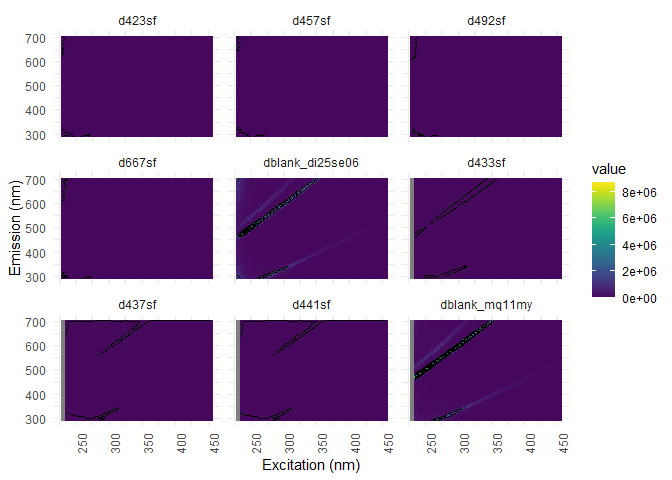
eem_overview_plot(eem_list, spp=9, contour = TRUE)
## [[1]]
## Warning: Removed 6294 rows containing non-finite values (stat_contour).
#Interpolation

eem_list <- eem_interp(eem_list, cores = cores, type = 1, extend = FALSE)
eem_overview_plot(eem_list, spp=9, contour = TRUE)
## [[1]]
## Warning: Removed 312 rows containing non-finite values (stat_contour).
Dilution corrections
In case of samples dilution, the data needs to be corrected with the appropriate factor.
dil_data <- meta["dilution"]# creation of the dataset containing the dilution factors
eem_list <- eem_dilution(eem_list,dil_data)#the correction
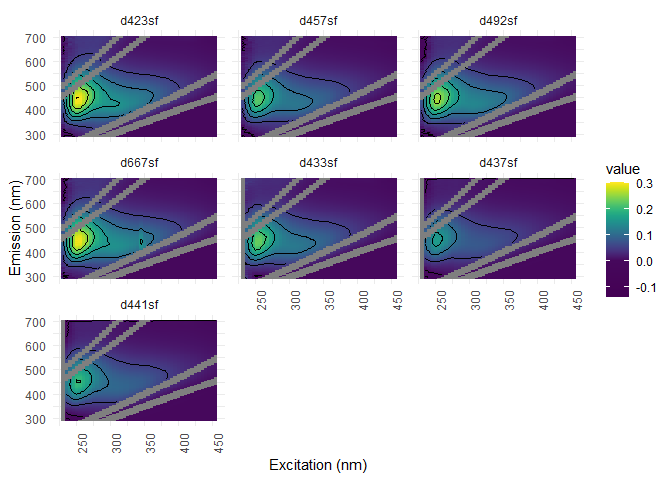
eem_overview_plot(eem_list, dil_data)
## [[1]]

##
## [[2]]
##
## [[3]]

##
## [[4]]
##
## [[5]]
##
## [[6]]
##
## [[7]]
Data smoothing
Depending on the instrument you are using smoothing your data could be a good idea for finding your fluorescence peaks. Although, this transformation is not suitable for the PARAFAC analysis. eem_smooth() smooth the fluorescence data by calculating rooling mean along excitation wavelength. In the following exemple, the rolling window is taking four nm at a time on the fluorescence data.
eem4peaks <- eem_smooth(eem_list, n = 4, cores = cores)#n sets the width of the rolling mean window in nm
Overview of the data before indices
This gives an overview of all the conditionning and transformation we performed on the data.
summary(eem_list)
##   sample ex_min ex_max em_min em_max is_blank_corrected is_scatter_corrected
## 1 d423sf    230    455    290    702               TRUE                 TRUE
## 2 d457sf    230    455    290    702               TRUE                 TRUE
## 3 d492sf    230    455    290    702               TRUE                 TRUE
## 4 d667sf    230    455    290    702               TRUE                 TRUE
## 5 d433sf    230    455    290    702               TRUE                 TRUE
## 6 d437sf    230    455    290    702               TRUE                 TRUE
## 7 d441sf    230    455    290    702               TRUE                 TRUE
##   is_ife_corrected is_raman_normalized
## 1             TRUE                TRUE
## 2             TRUE                TRUE
## 3             TRUE                TRUE
## 4             TRUE                TRUE
## 5             TRUE                TRUE
## 6             TRUE                TRUE
## 7             TRUE                TRUE
Choosing fluorescence peaks and indices
Smooth data is used here.
#Biological index, gives infos on autochtonous production/DOM from aquatic microbial sources;
#0.6-0.7 = More degraded DOM from terrestrial sources and
#>1 = freshly produced DOM by aquatic bacterias
bix <- eem_biological_index(eem4peaks)

#Coble peaks,
#B = protein-like tyrosine or tryptophan (microbial sources),
#T = protein-like tryptophan (microbial sources),
#A = humic substances (vascular plants sources),
#C = humic substances (vascular plants sources) and
#M = humic substances (autochtonous production sources)
coble_peaks <- eem_coble_peaks(eem4peaks)

#Fluorescence index, gives infos on DOM sources;
#1.7-2 = microbial sources,
#1.2-1.5 = soil and terrestrial plants sources
fi <- eem_fluorescence_index(eem4peaks)

#Humification index, gives infos on the humification degree;
#10-16 = terrestrial sources,
#<4 = autochtonous sources
hix <- eem_humification_index(eem4peaks, scale = TRUE)
#creation of the data table
indices_peaks <- bix %>%
  full_join(coble_peaks, by = "sample") %>%
  full_join(fi, by = "sample") %>%
  full_join(hix, by = "sample")

#data table
indices_peaks
##   sample       bix           b          t         a          m          c
## 1 d423sf 0.7238682 0.036238767 0.06222814 0.2799546 0.14974696 0.11645331
## 2 d457sf 0.6858719 0.023536584 0.04106616 0.2082118 0.11265412 0.08778000
## 3 d492sf 0.6869648 0.027140701 0.04730339 0.2413028 0.13198615 0.10493114
## 4 d667sf 0.6839838 0.031426888 0.05391093 0.2774084 0.14513535 0.13263827
## 5 d433sf 0.6941625 0.012110049 0.03792344 0.2147849 0.11547600 0.09000859
## 6 d437sf 0.6678838 0.006024978 0.02159146 0.1516322 0.07649198 0.06366574
## 7 d441sf 0.6670705 0.007355762 0.02692251 0.1882532 0.09387812 0.07938853
##         fi       hix
## 1 1.151716 0.8805637
## 2 1.143778 0.8923698
## 3 1.161794 0.8949828
## 4 1.139740 0.8965758
## 5 1.155606 0.9143584
## 6 1.116053 0.9420593
## 7 1.108152 0.9395073
Absorbance indices
Different absorbance indices can give different informations about the DOM sources. Here is the most commonly used:
- a254: CDOM absorption coefficient
- SR: Slope ratio; a high ratio means a low molecular weight and vice-versa
To calculate the aromaticity SUVA~254~ index: a254/DOC (mg/l)
slope_parms <- abs_parms(absorbance, cuvl = 1, cores = cores) #indices calculations
## Warning: `funs()` was deprecated in dplyr 0.8.0.
## Please use a list of either functions or lambdas:
##
##   # Simple named list:
##   list(mean = mean, median = median)
##
##   # Auto named with `tibble::lst()`:
##   tibble::lst(mean, median)
##
##   # Using lambdas
##   list(~ mean(., trim = .2), ~ median(., na.rm = TRUE))
## This warning is displayed once every 8 hours.
## Call `lifecycle::last_lifecycle_warnings()` to see where this warning was generated.
slope_parms #indices
##   sample      a254     a300    E2_E3    E4_E6   S275_295   S350_400   S300_700
## 1 d423sf 13.869423 6.341582 7.275041 54.45985 0.01693705 0.01767518 0.01757271
## 2 d433sf 11.629678 5.354673 7.195549 67.97273 0.01685673 0.01775750 0.01764950
## 3 d437sf  6.323142 2.836798 7.235020 39.38501 0.01750176 0.01674770 0.01719949
## 4 d441sf  7.703282 3.396527 7.572209 39.06406 0.01776943 0.01723729 0.01747484
## 5 d457sf 10.051932 4.654212 7.091301 71.26347 0.01675176 0.01752695 0.01741157
## 6 d492sf 11.652366 5.424564 7.060283 73.15475 0.01665879 0.01754663 0.01743985
## 7 d667sf 12.048233 5.542739 7.063998 35.38728 0.01648855 0.01797665 0.01702009
##          SR
## 1 0.9582393
## 2 0.9492738
## 3 1.0450242
## 4 1.0308717
## 5 0.9557717
## 6 0.9494014
## 7 0.9172203