PARAFAC part 2 : PARAFAC Analysis and model validation
Jade Dormoy-Boulanger and Mathieu Michaud
May 2022
- Before starting
- drEEM dataset importation
- Sample set wavelength ranges
- Find and remove noise in the EEMs
- The real PARAFAC starts
- Correlation verification between components
- Find and remove outliers
- Rerun the model with more precision
- Results plots
- Plots of the samples and their residue
- Half-split analysis
- Model formatting
- Exporting and interpreting the model
A tridimensional approach based on emission and excitation matrices (EEMs) can be produced with multiple spectral emission data collected successively with increasing excitation wavelength. The parallel factor analysis (PARAFAC) then allows to detect emission and excitation spectra produced by fluorophores that seems to be present in all the samples with the EEMs. The dissolved organic matter (DOM) components, by the fluorophores presence, can then be identified and quantified. Once they are identified, fluorophores and their according components can be associated with a production process, a molecule category and probable source.
There is also noe an open database to compare your PARAFAC results with others from literature (Open Fluor): https://doi:10.1039/c3ay41935e
This is an adaptation from a tutorial from Matthias Pucher, who is the staRdom developper, called “PARAFAC analysis of EEM data to separate DOM components in R”. We will use the example datasets contained within the staRdom package for this tutorial, but we also tried the method with real data as well, and we confident about the efficiency of the codes.
Link for Matthias Pucher tutorial: https://cran.r-project.org/web/packages/staRdom/vignettes/PARAFAC_analysis_of_EEM.html
The R method for PARAFAC and fluorescence indices is equvalent to the Matlab method, as this paper from Pucher et al. (2019) demonstrate it: https://doi.org/10.3390/w11112366
Part 2: PARAFAC
Selecting a PARAFAC model is an iterative process that can ask a lot of time and computer effort. We have test the mean calculation time for the first PARAFAC model of this excercice on different laptops and the results were out in between 4 min and 2 min 30. It is for this exact reason that this workshop is not in live coding.
Before starting
The first step is to install and load the staRdom and to check how many cores your computer have. The best calculation speed is acheived by setting the number of cores within somme of the most demanding function that we will be using. We will also need the following packages: dplyr, tidyr and eemR (eemR is installed with the staRdom package installation).
#packages loading
library(staRdom)
library(dplyr)
library(tidyr)
library(eemR)
library(knitr)
#speed calculation optimization
cores <-detectCores(logical = FALSE) # how many cores
cores # I have 6 cores
## [1] 4
drEEM dataset importation
#Name creation for temporary file
dreem_raw <- tempfile()

# Downloading drEEM data from Matlab repertory
download.file("http://models.life.ku.dk/sites/default/files/drEEM_dataset.zip",dreem_raw)

#"unzip" MatLab data
dreem_data <- unz(dreem_raw, filename="Backup/PortSurveyData_corrected.mat", open = "rb") %>%
  R.matlab::readMat()

# erase temporary path to the data since we do not need it anymore
unlink(dreem_raw)

# creation of a eemlist object
eem_list <- lapply(dreem_data$filelist.eem, function(file){
  n <- which(dreem_data$filelist.eem == file)
  file <- file %>%
    gsub("^\\s+|\\s+$", "", .) %>% # erase space in the file names
    sub(pattern = "(.*)\\..*$", replacement = "\\1", .) # erase extensions from file names
  eem <- list(file = paste0("drEEM/dataset/",file),sample = file,x = dreem_data$XcRU[n,,] %>%
  as.matrix(),ex = dreem_data$Ex %>% as.vector(), em = dreem_data$Em.in %>%
  as.vector(), location = "drEEM/dataset/")
  class(eem) <- "eem"
  attr(eem, "is_blank_corrected") <- TRUE
  attr(eem, "is_scatter_corrected") <- FALSE
  attr(eem, "is_ife_corrected") <- TRUE
  attr(eem, "is_raman_normalized") <- TRUE
  attr(eem, "manufacturer") <- "unknown"
  eem
}) %>%
  `class<-`("eemlist")

# add a prefix "d" to the file names, because R doesn't like when they start with a number
eem_names(eem_list) <- paste0("d",eem_names(eem_list))

#For this tutorial with drEEM dataset, we need to remove samples containing "bl" and  "0A" in their name
ol <- function(x){x==("bl") | x == "0A"}
extract <- dreem_data$sites %>% unlist() %>% ol() %>% which()
eem_list <- eem_list %>% eem_extract(extract)
## Removed sample(s): d0739sfK d0740sfK d0741sfK d0742sfK d0744sfK d1025sf
d1026sf d1027sf d1034sf d1036sf d1344sf d1345sf d1346sf d1348sf d1431sf d1433sf
Now that we have our dataset, it’s almost ready to use. The last step is to remove scattering.
eem_list <- eem_rem_scat(eem_list, remove_scatter = c(TRUE, TRUE, TRUE, TRUE),
remove_scatter_width = c(15,15,18,19), interpolation = F, cores = cores)
After that step, it is always best to check once again our dataset before going through the PARAFAC analysis with the eem_checkdata() function (not shown here)
If eem_checkdata() indicates to much NAs, there is two ways of improving the PARAFAC reliability: interpolate them or using an increased initiation number of start (we’ll see how to do that later in the tutorial). But for now, we will interpolate de NAs in the very next step.
Sample set wavelength ranges
For PARAFAC analysis, all samples must have similar paired wavelength. To acheived that, there is two methods:
- eem_extend2largest(), that add NAs into samples with smaller wavelength than the maximum in the whole dataset. Those NAs, can also be interpolated as well.
- eem_red2smallest() that remove wavelength not present in at least on sample in the dataset.
If you have a big dataset, we advise to use eem_red2smallest() in order to avoid interpolation if not needed. If you have a small dataset, use eem_extend2largest() instead.
eem_extend2largest(eem_list, interpolation = T)

#as the result is very large, it is not shown here
Find and remove noise in the EEMs
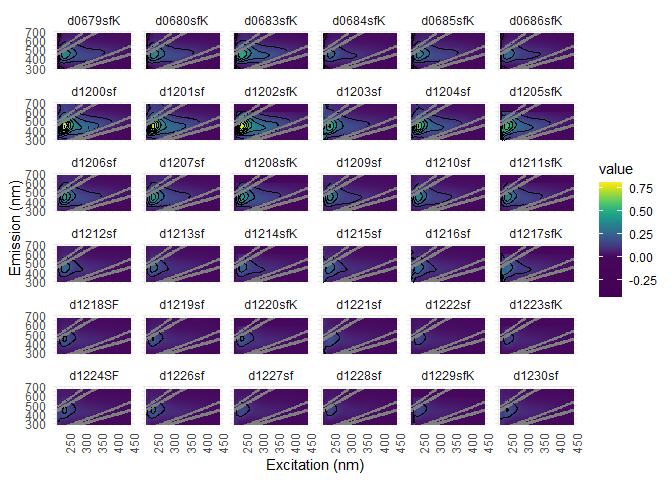
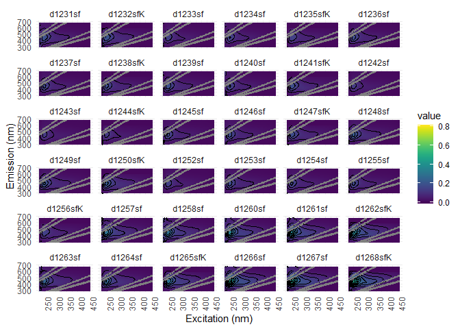
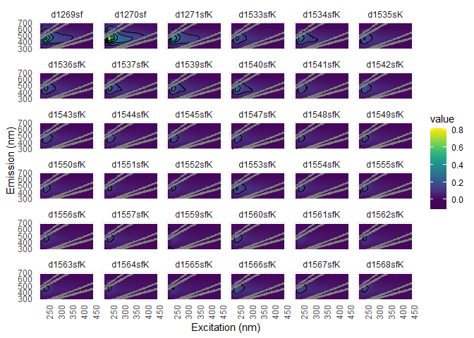
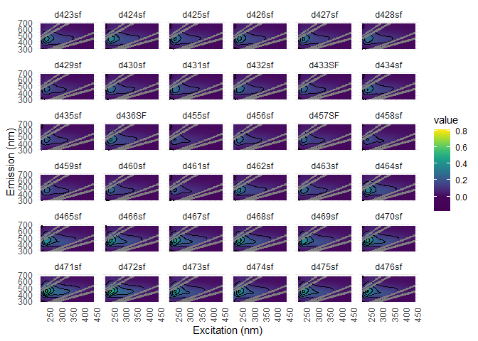
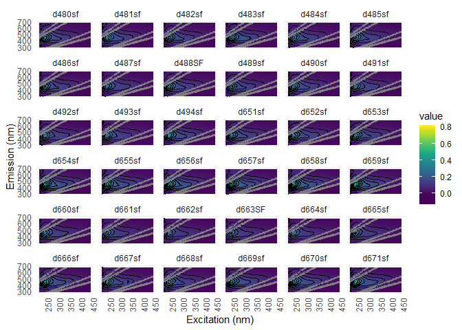
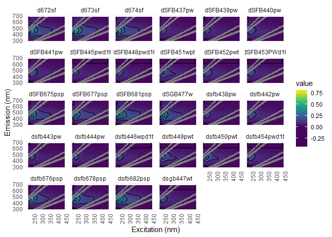
Visualization is a good way to find noise into EEMs. You can use eem_overview_plot() to do just that.
eem_overview_plot(eem_list, contour = T, spp=36)
## [[1]]
##
## [[2]]
##
## [[3]]
##
## [[4]]
##
## [[5]]
##
## [[6]]
The following functions, as shown in the PARAFAC part 1 workshop, can help removing the unwanted noise in your dataset:
- eem_extract(): remove entire sample by name or number
- eem_range(): remove data outside a given range of wavelength in the whole dataset
- eem_exclude(): remove data from the dataset according to a predetermined list
- eem_rem_scat() et eem_remove_scattering: remove Raman and Rayleigh peaks scattering. the first function allows to remove all the scattering at once, while the second remove one type of scattering at a time.
-
eem_interp(): offers several interpolation methods following the integrated function used:
- type = 0, NAs will be replaced by 0
- type = 1, preferred method, interpolation spline
- type = 2, interpolation from emission and excitation wavelength and their subsequent mean
- type = 3, interpolation from excitation wavelength
- type = 4, linear interpolation from emission and excitation wavelength and their subsequent mean
If the type = 1 interpolation method gives weird pattern in the graphs, then try another method.
To have a better idea of of the scattering removal through vizualisation, here is an exemple with sample d667sf. In order to extract that sample only from the dataset, we’ll use the experssion ^dd7sf$, where ^ stands fro the beginning of the string and $ the end. If these operator are not used, you’ll risk to extract every sample that contains these numbers in their name.
eem_list %>%
  eem_extract(sample = "^d667sf$", keep = TRUE) %>%
  ggeem(contour = TRUE)
## Extracted sample(s): d667sf
## Warning: Removed 930 rows containing non-finite values (stat_contour).
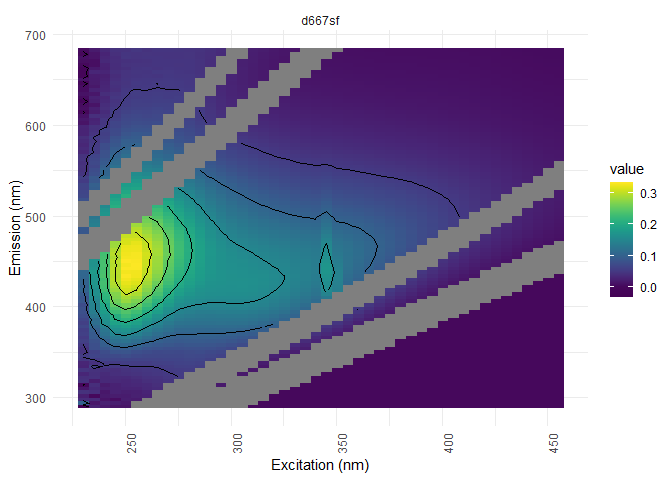
You can here see noise under 250 nm of excitation and above 580 nm of emission (looks like waves). This noise can be remove from the dataset with the following command:
eem_list <- eem_list %>%
  eem_setNA(sample = 176, ex = 345:350, interpolate = FALSE) %>%
  eem_setNA(em = 560:576, ex = 280:295, interpolate = FALSE)

# NAs interpolation following the noise removal
eem_list <- eem_interp(eem_list, type = 1, extend = FALSE, cores = cores)
The real PARAFAC starts
WARNING! This workshop results are not optimal. Please consider only the path and not the results. Do not consider the results!
It is beyond crucial to find the right number of components that suits your PARAFAC model in order to have a good liability. If the analysis has too much components, then the risk of one component being separated in two is increased. On the opposite, a too small number of components can lead to a lost of information. To help find the suitable number, we can calculate and compare a serie of PARAFAC models. In this workshop, five models from 3 to 7 components will be calculated and compared.
In order to optimize the components and to reduce functional residual errors, PARAFAC is based on a alternative least-squared algorithm.Depending on the random start value, different minimum of residual error can be found. To have a global minimum, a defined number of initialization nstart is used to separate model calculations. the model with the smallest residual error is than used to going through the PARAFAC analysis. For the following example, 25 is a good start, but for more in depth analysis, we suggest a highier number (e.g. 50).
Some of these random initialization can not converge, but if enough model converge, then the results will be reliable. If there is less than 50% of convergence, the eem_parafac() function will deliver a warning. In that case, we advise to increase the number of nstart.
You can also optimize the computation speed by specifying the number of your computer’s core to the eem_parafac() function with the argument cores.
Also, a high number of maximum iteration maxit and a low tolerance ctol can improve the liability of you model, but will also increase the processing time. For the final model, a tolerance between 10^-8^ et 10^-10^ is suitable and should never be highier than 10^-6^.
In this excercice, we’ll also have a non-negative fluorescence constraint (nonneg). Several constraints can be imposed to the model with the const argument from the eem_parafac() function. The more used are the following:
- uncons: no constraint
- nonneg: no negative values
- uninon: unimodal non-negative values
For more constraints, you can consult the complete list of available argument with the command CMLS::const().
At last, PARAFAC modes can be scaled so there maximum is 1, in order to improve the visualization within the plots. This is automaticallydone with mode A (the samples). For the inequality of the fluorescence peaks heights, the eempf_rescaleBC() function will rescale the B mode (emission wavelength) and the C mode (excitation wavelength) to also improve the plots. Other functions are also available and described in the Matthias Pucher tutorial: https://cran.r-project.org/web/packages/staRdom/vignettes/PARAFAC_analysis_of_EEM.html
# minimum of components
dim_min <- 3

# maximum of components
dim_max <- 7

#number of similar models from which the best is picked
nstart <- 25

#maximum number of iterations within the PARAFAC model
maxit = 5000

#tolerance of the model
ctol <- 10^-6

# Models calculation, one for each number of component. Warnings will pop to increased nstart...will be done in the last steps
pf1n <- eem_parafac(eem_list, comps = seq(dim_min,dim_max), normalise = FALSE,
const = c("nonneg", "nonneg", "nonneg"), maxit = maxit, nstart = nstart,
ctol = ctol, cores = cores)

#rescaling of the B and C modes
pf1n <- lapply(pf1n, eempf_rescaleBC, newscale = "Fmax")
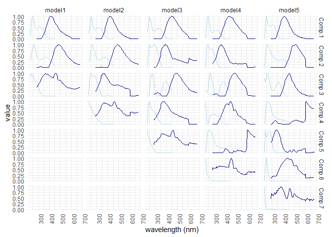
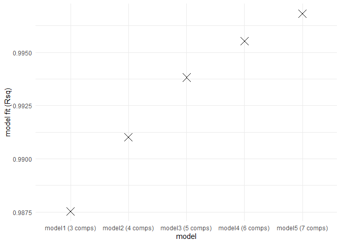
eempf_compare() will allows to compare via plots, all the model we just created. The first one are the fits, or R^2^, the second and third ones are different representation of all the models. In the third one, dark lines are emission wavelength and the pale ones are excitation wavelength. Keep in mind that we want a well adjusted fit (high R^2^), but not over adjusted (R^2^ higher above 1). In this case , the fourth model (6 components) seems to be the best one.
eempf_compare(pf1n, contour = TRUE)


## [[1]]
##
## [[2]]

##
## [[3]]

# Please note that the function will produce 6 plots (two times the same plots) and we do not know why.
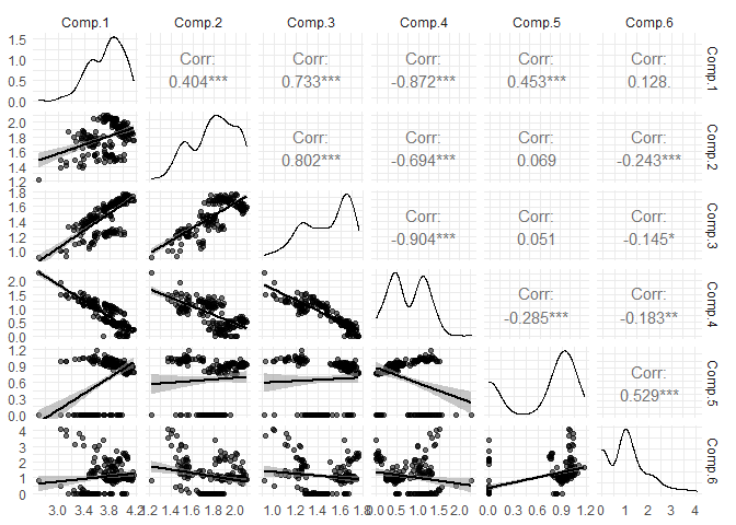
Correlation verification between components
The PARAFAC algorithm assumes, by default, no correlation between components. Although, if there is a lot a variability between the different dissolved organic carbon concentrations in the samples, the chance of having correlation increased. To avoid any problems, samples can be normalized. Keep in mind, we have selected model 4.
# verification table for correlation between components
eempf_cortable(pf1n[[4]], normalisation = FALSE)
##           Comp.1    Comp.2    Comp.3     Comp.4    Comp.5     Comp.6
## Comp.1 1.0000000 0.9653698 0.8469767  0.4780113 0.7160760  0.3238472
## Comp.2 0.9653698 1.0000000 0.7399814  0.6485079 0.7233542  0.1864222
## Comp.3 0.8469767 0.7399814 1.0000000  0.1944432 0.4403899  0.2968199
## Comp.4 0.4780113 0.6485079 0.1944432  1.0000000 0.6094110 -0.2176126
## Comp.5 0.7160760 0.7233542 0.4403899  0.6094110 1.0000000  0.4116712
## Comp.6 0.3238472 0.1864222 0.2968199 -0.2176126 0.4116712  1.0000000
#verification plots for correlation between components
eempf_corplot(pf1n[[4]], progress = FALSE, normalisation = FALSE)
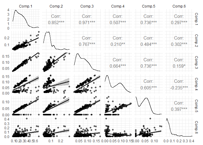
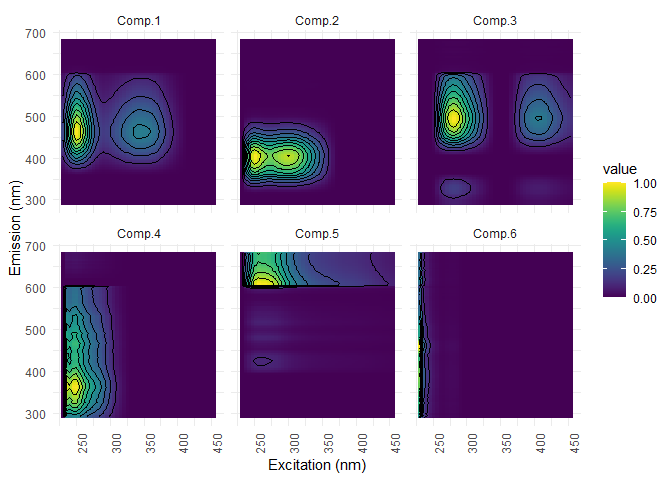
As some components are highly correlated, we will run the model again, but with normalized data. Further into the PARAFAC analysis, normalization will automatically be removed by multiplying mode A by the normalization factor for the plots’ and results’ exportation.
#new PARAFAC models with normalized data. Several warning will be displayed, asking for increasing nstart number...
# this will be done at the end...
pf2 <- eem_parafac(eem_list, comps = seq(dim_min,dim_max), normalise = TRUE, const = c("nonneg", "nonneg", "nonneg"),
maxit = maxit, nstart = nstart, ctol = ctol, cores = cores)
#rescaling mode B and C to a fluorescence maximum of 1 for each component
pf2 <- lapply(pf2, eempf_rescaleBC, newscale = "Fmax")
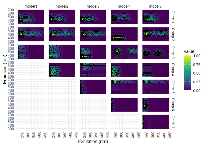
#new normalized models
eempf_plot_comps(pf2, contour = TRUE, type = 1)

Find and remove outliers
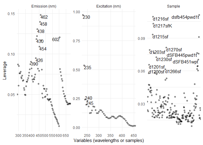
Leverage caused by outliers can decreased PARAFAC model liability by pulling the analysis toward those values. The leverage can be corrected by removing outliers from the dataset. To do that, there is two methods:
-
eempf_leverage() allows to calculate the leverage and eem_leverage_plot(), to create 3 plots showing the outliers. The outliers can then be selected and removed. In the plots we just created, they will appear above all the others values. Afterward, we can just create a list containing these outliers and exclude them from the dataset. This method will be shown in this workshop.
-
Following the leverage calculation with eempf_leverage(), eempf_leverage_ident() will create 3 interactive plots allowing you to simply click on the outliers. To change plot and eventually exit the interactive environment, you have to press the esc key on your keybord. If you use the following command to create your interactive plots, your outliers will be saved in an object called “exclude”:
exclude <- eempf_leverage_ident(cpl,qlabel=0.1)
#leverage calculation
cpl <- eempf_leverage(pf2[[4]])
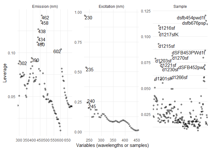
#plots displaying outliers
eempf_leverage_plot(cpl,qlabel=0.1)
#exclusion list creation

exclude <- list("ex" = c(),
                "em" = c(),
                "sample" = c("dsfb676psp","dsgb447wt")
)

#outliers exclusion from dataset
eem_list_ex <- eem_exclude(eem_list, exclude)
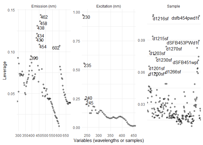
Following the outliers removal, we have to run again a PARAFAC model and check again for outliers.
#new PARAFAC models with normalized data. Several warning will be displayed, asking for increasing nstart number...
#this will be done at the end...
pf3 <- eem_parafac(eem_list_ex, comps = seq(dim_min,dim_max), normalise = TRUE,
maxit = maxit, nstart = nstart, ctol = ctol, cores = cores)
pf3 <- lapply(pf3, eempf_rescaleBC, newscale = "Fmax")

#visualization
eempf_plot_comps(pf3, contour = TRUE, type = 1)
#check again for outliers
eempf_leverage_plot(eempf_leverage(pf3[[4]]),qlabel=0.1)
Rerun the model with more precision
As previously mentioned a higher precision called for more calculation time. For this reason, tolerance is decreased only in the last step. We will only rerun the model 4 (6 components), but with the argument strictly_converging = TRUE to deduce a significant number of converging models. If you use = FALSE, make sure the ratio of converging model is ok and select the best model possible (we do not recommend this option!).
#Lower tolerance
ctol <- 10^-8

#Number of similar model from wich the best is selected
nstart <- 25

#iteration number for the PARAFAC analysis
maxit = 10000

#new model creation
pf4 <- eem_parafac(eem_list_ex, comps = 6, normalise = TRUE,
  const = c("nonneg", "nonneg", "nonneg"), maxit = maxit, nstart = nstart,
  ctol = ctol, output = "all", cores = cores, strictly_converging = TRUE)

pf4 <- lapply(pf4, eempf_rescaleBC, newscale = "Fmax")

#checking for convergence
eempf_convergence(pf4[[1]])
## Calculated models:  25
## Converging models:  25
## Not converging Models, iteration limit reached:  0
## Not converging models, other reasons:  0
## Best SSE:  8240.529
## Summary of SSEs of converging models:
##    Min. 1st Qu.  Median    Mean 3rd Qu.    Max.
##    8241    8242    8242    8339    8340    9892
#checking for outliers
eempf_leverage_plot(eempf_leverage(pf4[[1]]))
#checking for correlation
eempf_corplot(pf4[[1]], progress = FALSE)
Repeat the creation steps until you are completely satisfied with your results
Results plots
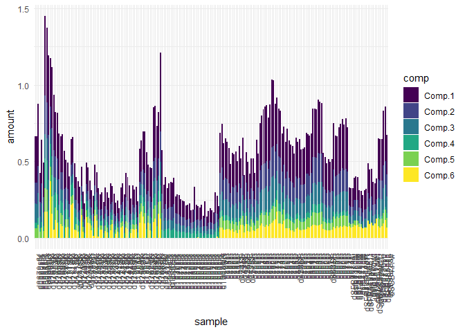
The following plots show two crucial informations: The first plot shows the components shape and gives infos on the composition and the second plot provides their loading in each of your sample.
eempf_comp_load_plot(pf4[[1]], contour = TRUE)
## [[1]]
##
## [[2]]
Plots of the samples and their residue
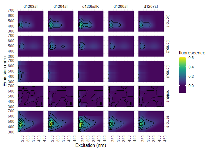
Columns represents samples and lines the components (3), the residue. We used pf3, since this model still has the outliers, that could be of interest.
eempf_residuals_plot(pf3[[1]], eem_list, select = eem_names(eem_list)[10:14], cores = cores, contour = TRUE)
## [[1]]
Half-split analysis
The half-split analysis check for the model’s stability. Data is recombined in 6 different ways and the results should be similar. This is a very long analysis!
#half-split analysis
sh <- splithalf(eem_list_ex, 6, normalise = TRUE, rand = FALSE, cores = cores,
  nstart = nstart, strictly_converging = TRUE, maxit = maxit, ctol = ctol)

#plot
splithalf_plot(sh)
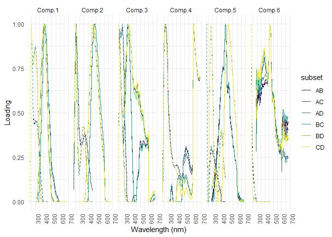
The Tucker congruence factor is also a tool to test the similarity. A factor of 1 is a perfect similarity.
#table creation
tcc_sh_table <- splithalf_tcc(sh)

#table
tcc_sh_table
##    component   comb    tcc_em    tcc_ex
## 1     Comp.1 ABvsCD 0.9644244 0.9218130
## 2     Comp.1 ACvsBD 0.9598692 0.9289599
## 3     Comp.1 ADvsBC 0.9347265 0.9474255
## 4     Comp.2 ABvsCD 0.9427617 0.9806922
## 5     Comp.2 ACvsBD 0.9390894 0.9830222
## 6     Comp.2 ADvsBC 0.9615423 0.9437636
## 7     Comp.3 ABvsCD 0.8996063 0.8780016
## 8     Comp.3 ACvsBD 0.9025069 0.8913317
## 9     Comp.3 ADvsBC 0.5893373 0.9821453
## 10    Comp.4 ABvsCD 0.9954748 0.9512482
## 11    Comp.4 ACvsBD 0.9966581 0.9750486
## 12    Comp.4 ADvsBC 0.9158385 0.8808372
## 13    Comp.5 ABvsCD 0.5598656 0.9432919
## 14    Comp.5 ACvsBD 0.5840912 0.9516407
## 15    Comp.5 ADvsBC 0.9948352 0.9694507
## 16    Comp.6 ABvsCD 0.9316002 0.9896928
## 17    Comp.6 ACvsBD 0.9434008 0.9938588
## 18    Comp.6 ADvsBC 0.9511401 0.9810148
Other validation analysis are available and described in the Matthias Pucher tutorial at section 8.13: https://cran.r-project.org/web/packages/staRdom/vignettes/PARAFAC_analysis_of_EEM.html
Model formatting
Naming the model and the different components
Fomatting your plot is very important for the model comprehension and visualization.
# obtain the current models name (there is none!)
names(pf3)
## NULL
# Naming the different models (careful, the number of models must be equal to the number of names)
names(pf3) <- c("3 components", "4 components xy","5 components no outliers","6 components","7 components")

names(pf3)
## [1] "3 components"             "4 components xy"
## [3] "5 components no outliers" "6 components"
## [5] "7 components"
# Obtain the current components name for the final model
eempf_comp_names(pf4)
## [[1]]
## [1] "Comp.1" "Comp.2" "Comp.3" "Comp.4" "Comp.5" "Comp.6"
#renaming the different components name in the final model
eempf_comp_names(pf4) <- c("A4","B4","C4","D4","E4","F4")
#renaming the components name in several models at a time (ex: pf3)
eempf_comp_names(pf3) <- list(c("A1","B1","C1"),
c("humic","T2","whatever","peak"),
c("rose","peter","frank","dwight","susan"),
c("A4","B4","C4","D4","E4","F4"),
c("A5","B5","C5","D5","E5","F5","G5"))
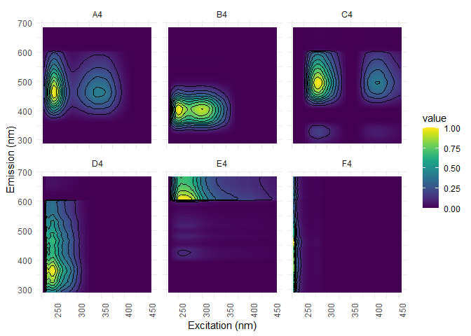
#Final model's plot with new names
pf4[[1]] %>%
ggeem(contour = TRUE)
Exporting and interpreting the model
Please note that the Matthias Pucher tutorial offers others possibilities than the one presented in this workshop: https://cran.r-project.org/web/packages/staRdom/vignettes/PARAFAC_analysis_of_EEM.html
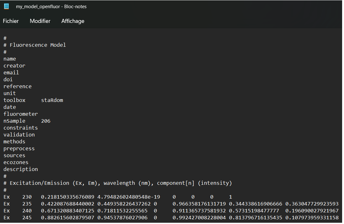
Comparing your results with the openfluor.org database
eempf_openfluor() can export your PARAFAC model into a txt file that can be uploaded on openfluor.org and compared to other results from the literature. Be careful to check the exported headers, since some infos are not automatically filled.
eempf_openfluor(pf4[[1]], file = "my_model_openfluor.txt")
## An openfluor file has been successfully written. Please fill in missing header fields manually!

Create the PARAFAC report
The report created using eempf_report() contains important infos from your model, as well as the results. The report will be exported under a html format. You can also indicate what information you want to display in the report.
eempf_report(pf4[[1]], export = "parafac_report.html", eem_list = eem_list_ex, shmodel = sh, performance = TRUE)
##
##
## processing file: PARAFAC_report.Rmd
## output file: PARAFAC_report.knit.md
##
## Output created: parafac_report.html
Model exportation
eempf_export() allows to export a csv file containing your results matrices.
eempf_export(pf4[[1]], export = "parafac_report.csv")
The end