Introduction to Python
Charles Martin
October 2022
Setup
Python is a general programming language. Unlike R or MATLAB, it was not designed specifically for data analysis and visualization. This is why most of the code that we will use today comes from code libraries that have been created for these specific uses.
Although many operating systems come with a version of Python pre-installed (including Ubuntu, MacOS, etc.), its configuration, the installation of libraries, etc. can be relatively perilous for a beginner.
This is why for this workshop, we will work with Python on Google Colab (https://colab.research.google.com/). Colab is a service offered by Google, where you can create a Jupyter notebook in which you can mix code (Python and others) and text (in Markdown format). As all the necessary software is already pre-installed, we will save a LOT of configuration time.
We can also, immediately, check that our notebook works well by launching a first test command
print("Hello, World!")Hello, World!
That said, if you ever want to work directly on your computers, I advise you to install Python through a library manager (eg Anaconda). This way of doing things will allow you, among other things, to avoid version conflicts between your different projects.
Python basics
Python can be used as a calculator
1+123*515The exponents are different from those we often see (i.e. 2^5)
2**8256Results can be saved in an object
mon_resultat = 3+2mon_resultat*630Lists
We won't have time here (obviously!) to explore all the possible data structures and functions of Python.
We will still take the time to get to grips with one, which should be the most useful, namely the lists
especes = ['bouleau','érable','chêne']The various elements of a list can be accessed from their index, which starts at 0 (rather than 1, it's an old programmer war)
print(especes[0])bouleau
List elements can also be modified
especes[2] = 'sapin'
print(especes)
['bouleau', 'érable', 'sapin']
And added
especes.append('épinette')
print(especes)
['bouleau', 'érable', 'sapin', 'épinette']
Notice in the previous example the use of the syntax object.function.
We won't go too deep into these details today, but since Python is an object-oriented language, each of the objects has a series of actions (functions) they can perform and associated data. To access these, we use the notation object.method or object.data.
You can also delete items, either by position, or by their value directly
del especes[1]
especes.remove('bouleau')
print(especes)
['sapin', 'épinette']
Note that if you use the by-value method, only the first value will be removed.
Loops and functions
To automate things in Python, we can, among other things, use functions and loops
We can for example print the name of each species like this
for espece in especes :
  print(espece)
sapin
épinette
Note that, in Python, whitespace usage is part of the language structure, i.e. it is not purely cosmetic as in other languages.
All text that is indented is part of the loop. No need for braces, parentheses, etc. It's very elegant!
We can also create a function that, for example, checks if our species is a spruce
def cest_une_epinette(x) :
  if x == 'épinette' :
    return "oui"
  else :
    return "non"
for espece in especes :
print(espece)
print(cest_une_epinette(espece))sapin
non
épinette
oui
Dictionaries
Another important Python data structure is called data dictionaries. While lists only contain series of values, dictionaries contain pairs of key-value associations.
They are defined using braces rather than square parentheses.
infos = {'nom' : 'charles', 'age' : 42, 'ville': 'Trois-Rivières'}
infos
{'nom': 'charles', 'age': 42, 'ville': 'Trois-Rivières'}We still access the elements of a dictionary using square parentheses
infos['nom']{"type":"string"}We can get all the keys or values like this:
print(infos.keys())
print(infos.values())
dict_keys(['nom', 'age', 'ville'])
dict_values(['charles', 42, 'Trois-Rivières'])
It is possible to combine different data structures to form complex objects, such as a list of dictionaries:
repondants = [
    {'nom' : 'Charles', 'language' : 'R'},
    {'nom' : 'Alex', 'language' : 'Python'}
]

for repondant in repondants :
  print(repondant['nom']+' préfère ' + repondant['language'])
Charles préfère R
Alex préfère Python
Vectorized operations
Unlike many languages created expressly for data analysis, Python is not a naturally vectorized language.
If we are preparing a list and we want to multiply all its items by 2, we can NOT do this:
liste = [1,2,3,4]liste*2[1, 2, 3, 4, 1, 2, 3, 4]We could obviously work around the problem with loops
nouvelle_liste = []

for chiffre in liste :
  nouvelle_liste.append(chiffre*2)

nouvelle_liste
[2, 4, 6, 8]Python has a more compact notation for this kind of problem : list comprehension
[x * 2 for x in liste][2, 4, 6, 8]It is a very compact structure, allowing to create a list from another list.
Finally, if you have a lot of vector or matrix algebra to do, it will probably be easier to use the library provided for this purpose, which is called NumPy.
NumPy (and all the other libraries needed for the workshop) are already installed on Colab.
On your personal computers, we install NumPy by the command line (terminal), for example like this:
pip install numpy
In Python, when you activate a library, all the loaded code is associated with a prefix, which can be modified at the time of activation
import numpy as np

tableau = np.array([1,2,3,4])
print(tableau)
print(tableau*2)
[1 2 3 4]
[2 4 6 8]
matrice = np.array([[1,2,3,4],[5,6,7,8]])
print(matrice)
[[1 2 3 4]
[5 6 7 8]]
print(matrice.dot(tableau))[30 70]
Panda data frames
There is a library that manages data frames much more appropriately than lists or dictionaries when it comes to statistical analysis of data. This library is called pandas.
It takes its name from a common data structure in economics, PANel DAta.
import pandas as pdLoading and verifying data
The pandas function for loading data is called read_csv.
To simplify, we will load data directly available on the web
iris = pd.read_csv('https://raw.githubusercontent.com/mwaskom/seaborn-data/master/iris.csv')
iris| sepal_length | sepal_width | petal_length | petal_width | species | |
|---|---|---|---|---|---|
| 0 | 5.1 | 3.5 | 1.4 | 0.2 | setosa |
| 1 | 4.9 | 3.0 | 1.4 | 0.2 | setosa |
| 2 | 4.7 | 3.2 | 1.3 | 0.2 | setosa |
| 3 | 4.6 | 3.1 | 1.5 | 0.2 | setosa |
| 4 | 5.0 | 3.6 | 1.4 | 0.2 | setosa |
| ... | ... | ... | ... | ... | ... |
| 145 | 6.7 | 3.0 | 5.2 | 2.3 | virginica |
| 146 | 6.3 | 2.5 | 5.0 | 1.9 | virginica |
| 147 | 6.5 | 3.0 | 5.2 | 2.0 | virginica |
| 148 | 6.2 | 3.4 | 5.4 | 2.3 | virginica |
| 149 | 5.9 | 3.0 | 5.1 | 1.8 | virginica |
150 rows × 5 columns
If your data is in Excel format, there is also a read_excel function allowing you to read them directly, without going through the CSV format.
Once the data is loaded, it is important to check the contents our data, for example with the info method:
iris.info()<class 'pandas.core.frame.DataFrame'>
RangeIndex: 150 entries, 0 to 149
Data columns (total 5 columns):
# Column Non-Null Count Dtype
--- ------ -------------- -----
0 sepal_length 150 non-null float64
1 sepal_width 150 non-null float64
2 petal_length 150 non-null float64
3 petal_width 150 non-null float64
4 species 150 non-null object
dtypes: float64(4), object(1)
memory usage: 6.0+ KB
Sorting data
In ascending order
iris.sort_values('sepal_length')| sepal_length | sepal_width | petal_length | petal_width | species | |
|---|---|---|---|---|---|
| 13 | 4.3 | 3.0 | 1.1 | 0.1 | setosa |
| 42 | 4.4 | 3.2 | 1.3 | 0.2 | setosa |
| 38 | 4.4 | 3.0 | 1.3 | 0.2 | setosa |
| 8 | 4.4 | 2.9 | 1.4 | 0.2 | setosa |
| 41 | 4.5 | 2.3 | 1.3 | 0.3 | setosa |
| ... | ... | ... | ... | ... | ... |
| 122 | 7.7 | 2.8 | 6.7 | 2.0 | virginica |
| 118 | 7.7 | 2.6 | 6.9 | 2.3 | virginica |
| 117 | 7.7 | 3.8 | 6.7 | 2.2 | virginica |
| 135 | 7.7 | 3.0 | 6.1 | 2.3 | virginica |
| 131 | 7.9 | 3.8 | 6.4 | 2.0 | virginica |
150 rows × 5 columns
Or in descending order
iris.sort_values('sepal_length', ascending = False)| sepal_length | sepal_width | petal_length | petal_width | species | |
|---|---|---|---|---|---|
| 131 | 7.9 | 3.8 | 6.4 | 2.0 | virginica |
| 135 | 7.7 | 3.0 | 6.1 | 2.3 | virginica |
| 122 | 7.7 | 2.8 | 6.7 | 2.0 | virginica |
| 117 | 7.7 | 3.8 | 6.7 | 2.2 | virginica |
| 118 | 7.7 | 2.6 | 6.9 | 2.3 | virginica |
| ... | ... | ... | ... | ... | ... |
| 41 | 4.5 | 2.3 | 1.3 | 0.3 | setosa |
| 42 | 4.4 | 3.2 | 1.3 | 0.2 | setosa |
| 38 | 4.4 | 3.0 | 1.3 | 0.2 | setosa |
| 8 | 4.4 | 2.9 | 1.4 | 0.2 | setosa |
| 13 | 4.3 | 3.0 | 1.1 | 0.1 | setosa |
150 rows × 5 columns
Selecting rows
There are several ways to select rows or columns with pandas, but the most general way is to use the loc operator.
The latter can accept either a list of Boolean values, or labels or a sequence between two labels.
This operator also allows you to simultaneously select a list of columns AND rows in the same operation.
iris.loc[iris.species == "virginica"]| sepal_length | sepal_width | petal_length | petal_width | species | |
|---|---|---|---|---|---|
| 100 | 6.3 | 3.3 | 6.0 | 2.5 | virginica |
| 101 | 5.8 | 2.7 | 5.1 | 1.9 | virginica |
| 102 | 7.1 | 3.0 | 5.9 | 2.1 | virginica |
| 103 | 6.3 | 2.9 | 5.6 | 1.8 | virginica |
| 104 | 6.5 | 3.0 | 5.8 | 2.2 | virginica |
| 105 | 7.6 | 3.0 | 6.6 | 2.1 | virginica |
| 106 | 4.9 | 2.5 | 4.5 | 1.7 | virginica |
| 107 | 7.3 | 2.9 | 6.3 | 1.8 | virginica |
| 108 | 6.7 | 2.5 | 5.8 | 1.8 | virginica |
| 109 | 7.2 | 3.6 | 6.1 | 2.5 | virginica |
| 110 | 6.5 | 3.2 | 5.1 | 2.0 | virginica |
| 111 | 6.4 | 2.7 | 5.3 | 1.9 | virginica |
| 112 | 6.8 | 3.0 | 5.5 | 2.1 | virginica |
| 113 | 5.7 | 2.5 | 5.0 | 2.0 | virginica |
| 114 | 5.8 | 2.8 | 5.1 | 2.4 | virginica |
| 115 | 6.4 | 3.2 | 5.3 | 2.3 | virginica |
| 116 | 6.5 | 3.0 | 5.5 | 1.8 | virginica |
| 117 | 7.7 | 3.8 | 6.7 | 2.2 | virginica |
| 118 | 7.7 | 2.6 | 6.9 | 2.3 | virginica |
| 119 | 6.0 | 2.2 | 5.0 | 1.5 | virginica |
| 120 | 6.9 | 3.2 | 5.7 | 2.3 | virginica |
| 121 | 5.6 | 2.8 | 4.9 | 2.0 | virginica |
| 122 | 7.7 | 2.8 | 6.7 | 2.0 | virginica |
| 123 | 6.3 | 2.7 | 4.9 | 1.8 | virginica |
| 124 | 6.7 | 3.3 | 5.7 | 2.1 | virginica |
| 125 | 7.2 | 3.2 | 6.0 | 1.8 | virginica |
| 126 | 6.2 | 2.8 | 4.8 | 1.8 | virginica |
| 127 | 6.1 | 3.0 | 4.9 | 1.8 | virginica |
| 128 | 6.4 | 2.8 | 5.6 | 2.1 | virginica |
| 129 | 7.2 | 3.0 | 5.8 | 1.6 | virginica |
| 130 | 7.4 | 2.8 | 6.1 | 1.9 | virginica |
| 131 | 7.9 | 3.8 | 6.4 | 2.0 | virginica |
| 132 | 6.4 | 2.8 | 5.6 | 2.2 | virginica |
| 133 | 6.3 | 2.8 | 5.1 | 1.5 | virginica |
| 134 | 6.1 | 2.6 | 5.6 | 1.4 | virginica |
| 135 | 7.7 | 3.0 | 6.1 | 2.3 | virginica |
| 136 | 6.3 | 3.4 | 5.6 | 2.4 | virginica |
| 137 | 6.4 | 3.1 | 5.5 | 1.8 | virginica |
| 138 | 6.0 | 3.0 | 4.8 | 1.8 | virginica |
| 139 | 6.9 | 3.1 | 5.4 | 2.1 | virginica |
| 140 | 6.7 | 3.1 | 5.6 | 2.4 | virginica |
| 141 | 6.9 | 3.1 | 5.1 | 2.3 | virginica |
| 142 | 5.8 | 2.7 | 5.1 | 1.9 | virginica |
| 143 | 6.8 | 3.2 | 5.9 | 2.3 | virginica |
| 144 | 6.7 | 3.3 | 5.7 | 2.5 | virginica |
| 145 | 6.7 | 3.0 | 5.2 | 2.3 | virginica |
| 146 | 6.3 | 2.5 | 5.0 | 1.9 | virginica |
| 147 | 6.5 | 3.0 | 5.2 | 2.0 | virginica |
| 148 | 6.2 | 3.4 | 5.4 | 2.3 | virginica |
| 149 | 5.9 | 3.0 | 5.1 | 1.8 | virginica |
Note that, if only one column is accessed at a time and the column name is a valid Python identifier (no spaces, no accents, etc.), it can be accessed directly with a . variable rather than ['variable']
Selecting columns
The principle is the same for selecting columns. On the other hand, we must at this time specify which lines we want to obtain (or specify all the lines, like this)
iris.loc[:,["sepal_width", "species"]]| sepal_width | species | |
|---|---|---|
| 0 | 3.5 | setosa |
| 1 | 3.0 | setosa |
| 2 | 3.2 | setosa |
| 3 | 3.1 | setosa |
| 4 | 3.6 | setosa |
| ... | ... | ... |
| 145 | 3.0 | virginica |
| 146 | 2.5 | virginica |
| 147 | 3.0 | virginica |
| 148 | 3.4 | virginica |
| 149 | 3.0 | virginica |
150 rows × 2 columns
And as discussed, we can combine the two operations in the same command:
iris.loc[iris.species == "virginica",["sepal_width", "species"]]| sepal_width | species | |
|---|---|---|
| 100 | 3.3 | virginica |
| 101 | 2.7 | virginica |
| 102 | 3.0 | virginica |
| 103 | 2.9 | virginica |
| 104 | 3.0 | virginica |
| 105 | 3.0 | virginica |
| 106 | 2.5 | virginica |
| 107 | 2.9 | virginica |
| 108 | 2.5 | virginica |
| 109 | 3.6 | virginica |
| 110 | 3.2 | virginica |
| 111 | 2.7 | virginica |
| 112 | 3.0 | virginica |
| 113 | 2.5 | virginica |
| 114 | 2.8 | virginica |
| 115 | 3.2 | virginica |
| 116 | 3.0 | virginica |
| 117 | 3.8 | virginica |
| 118 | 2.6 | virginica |
| 119 | 2.2 | virginica |
| 120 | 3.2 | virginica |
| 121 | 2.8 | virginica |
| 122 | 2.8 | virginica |
| 123 | 2.7 | virginica |
| 124 | 3.3 | virginica |
| 125 | 3.2 | virginica |
| 126 | 2.8 | virginica |
| 127 | 3.0 | virginica |
| 128 | 2.8 | virginica |
| 129 | 3.0 | virginica |
| 130 | 2.8 | virginica |
| 131 | 3.8 | virginica |
| 132 | 2.8 | virginica |
| 133 | 2.8 | virginica |
| 134 | 2.6 | virginica |
| 135 | 3.0 | virginica |
| 136 | 3.4 | virginica |
| 137 | 3.1 | virginica |
| 138 | 3.0 | virginica |
| 139 | 3.1 | virginica |
| 140 | 3.1 | virginica |
| 141 | 3.1 | virginica |
| 142 | 2.7 | virginica |
| 143 | 3.2 | virginica |
| 144 | 3.3 | virginica |
| 145 | 3.0 | virginica |
| 146 | 2.5 | virginica |
| 147 | 3.0 | virginica |
| 148 | 3.4 | virginica |
| 149 | 3.0 | virginica |
Note that the original table is not affected by these operations. If we want to keep the result, we have to keep it in an object
iris.shape(150, 5)iris_modifie = iris.loc[iris.species == "virginica",["sepal_width", "species"]]iris.shape(150, 5)iris_modifie.shape(50, 2)Adding columns
iris.assign(ratio = iris.sepal_length / iris.petal_length)| sepal_length | sepal_width | petal_length | petal_width | species | ratio | |
|---|---|---|---|---|---|---|
| 0 | 5.1 | 3.5 | 1.4 | 0.2 | setosa | 3.642857 |
| 1 | 4.9 | 3.0 | 1.4 | 0.2 | setosa | 3.500000 |
| 2 | 4.7 | 3.2 | 1.3 | 0.2 | setosa | 3.615385 |
| 3 | 4.6 | 3.1 | 1.5 | 0.2 | setosa | 3.066667 |
| 4 | 5.0 | 3.6 | 1.4 | 0.2 | setosa | 3.571429 |
| ... | ... | ... | ... | ... | ... | ... |
| 145 | 6.7 | 3.0 | 5.2 | 2.3 | virginica | 1.288462 |
| 146 | 6.3 | 2.5 | 5.0 | 1.9 | virginica | 1.260000 |
| 147 | 6.5 | 3.0 | 5.2 | 2.0 | virginica | 1.250000 |
| 148 | 6.2 | 3.4 | 5.4 | 2.3 | virginica | 1.148148 |
| 149 | 5.9 | 3.0 | 5.1 | 1.8 | virginica | 1.156863 |
150 rows × 6 columns
Summarizing data
To get an overview of all the descriptive statistics of our data table, we can use the describe function
iris.describe()| sepal_length | sepal_width | petal_length | petal_width | |
|---|---|---|---|---|
| count | 150.000000 | 150.000000 | 150.000000 | 150.000000 |
| mean | 5.843333 | 3.057333 | 3.758000 | 1.199333 |
| std | 0.828066 | 0.435866 | 1.765298 | 0.762238 |
| min | 4.300000 | 2.000000 | 1.000000 | 0.100000 |
| 25% | 5.100000 | 2.800000 | 1.600000 | 0.300000 |
| 50% | 5.800000 | 3.000000 | 4.350000 | 1.300000 |
| 75% | 6.400000 | 3.300000 | 5.100000 | 1.800000 |
| max | 7.900000 | 4.400000 | 6.900000 | 2.500000 |
If we need finer control, we can specify functions and columns manually
iris.loc[:,['sepal_length', 'petal_length']].agg(['mean','min','max','count'])| sepal_length | petal_length | |
|---|---|---|
| mean | 5.843333 | 3.758 |
| min | 4.300000 | 1.000 |
| max | 7.900000 | 6.900 |
| count | 150.000000 | 150.000 |
We can also apply our summaries to specific groups
iris.groupby('species')[['sepal_length', 'petal_length']].mean()| sepal_length | petal_length | |
|---|---|---|
| species | ||
| setosa | 5.006 | 1.462 |
| versicolor | 5.936 | 4.260 |
| virginica | 6.588 | 5.552 |
Data visualization with matlplotlib
The classic module for data visualization with Python is called matplotlib. In general, people especially use the collection of functions named pyplot, which aims to replicate MATLAB's plotting interface in Python
import matplotlib.pyplot as pltExploring each variable variable individually
To create a frequency histogram, the function is called hist.
plt.hist('sepal_length', data = iris)(array([ 9., 23., 14., 27., 16., 26., 18., 6., 5., 6.]),
array([4.3 , 4.66, 5.02, 5.38, 5.74, 6.1 , 6.46, 6.82, 7.18, 7.54, 7.9 ]),
<a list of 10 Patch objects>)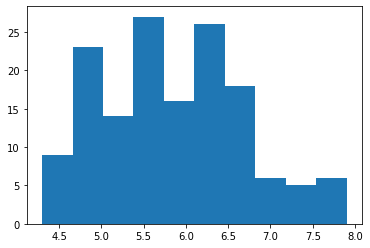
As matplotlib and pandas are extremely well integrated, there is, for most visualizations, a way to call them directly from the data frame
iris.sepal_length.plot.hist()<matplotlib.axes._subplots.AxesSubplot at 0x7f17e8c77a50>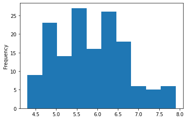
You can then make changes to this graph (or the previous one), then ask to display it again
iris.sepal_length.plot.hist()
plt.ylabel("Fréquence")
plt.xlabel("Longueur des sépales")
Text(0.5, 0, 'Longueur des sépales')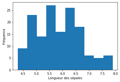
If you ever work with matplotlib in a script rather than on Jupyter, you will need to call plt.show() to display your plot. Here, Jupyter does it for you.
If our data is qualitative, we use a bar chart instead.
Unlike the previous example, here we must first calculate the counts for each class
iris.species.value_counts().plot.bar()<matplotlib.axes._subplots.AxesSubplot at 0x7f17e8b20150>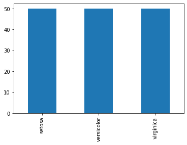
Exploring relationships between two variables
To look at the relationship between two quantitative variables, we of course have access to the classic scatter plot
iris.plot.scatter('petal_length', 'petal_width')<matplotlib.axes._subplots.AxesSubplot at 0x7f17e8af49d0>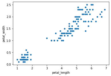
And I'll quickly show you how to change the color of the dots because I had a little trouble figuring out how to do it for a categorical variable.
The key is to first create a dictionary associating each species with a color.
Then when creating the graph, associate each species value with a color value with the map method.
couleurs = {'setosa':'red', 'virginica':'green', 'versicolor':'blue'}
iris.plot.scatter('petal_length','petal_width',c=iris.species.map(couleurs))
<matplotlib.axes._subplots.AxesSubplot at 0x7f17e8a8be90>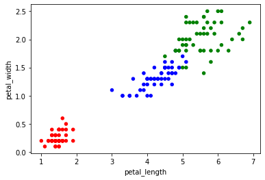
If you want to explore the relationship between a qualitative variable and a quantitative one, there is obviously the boxplot
iris.boxplot(column='sepal_length',by='species', grid = False)<matplotlib.axes._subplots.AxesSubplot at 0x7f17e89f8150>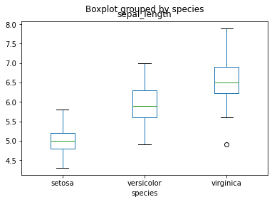
A hint of R
If you ever miss ggplot2, the entire library has been re-implemented in Python in the plotnine library.
Note that there are still some small nuances vs. the R code. You will not be able to directly copy and paste your code.
from plotnine import ggplot, aes,geom_point

ggplot(iris) + aes(x = "sepal_length", y = "sepal_width") + geom_point()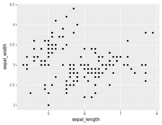
<ggplot: (8733791616949)>Statistical tests with scipy
Classic statistical tests in Python are provided by the collection of stats functions in the scipy module
from scipy import statsIf you want for example to apply a T test for unequal variance
stats.ttest_ind(
    iris.loc[iris.species == "virginica", 'petal_length'],
    iris.loc[iris.species == "setosa", 'petal_length'],
    equal_var = False
)
Ttest_indResult(statistic=49.98618625709594, pvalue=9.26962758534569e-50)If you want to measure a Pearson correlation (and get the corresponding p-value)
stats.pearsonr(
    iris.petal_length,
    iris.sepal_length
)
(0.8717537758865831, 1.0386674194498099e-47)Machine Learning with scikit-learn
Most Machine Learning algorithms are available in Python through the scikit-learn module
Example with a Random Forest
Here is how, for example, we could apply a Random Forest classification model to our data.
Note that we must first encode our qualitative variable in numeric so that the model understands it...
from sklearn.preprocessing import LabelEncoder

le = LabelEncoder()
Y = le.fit_transform(iris.species)

X = iris.loc[:,['sepal_length','sepal_width']]
We can then run the model and see how well it works!
from sklearn.ensemble import RandomForestClassifier

rf = RandomForestClassifier()
rf.fit(X,Y)

rf.score(X,Y)0.9266666666666666Example with a PCA
The sklearn library contains a function to calculate a principal component analysis named PCA in the decomposition module. PCA is there, since it is, in data science jargon, an unsupervised learning technique.
Note that the function always applies its calculation to the variance/covariance matrix. You will have to center-reduce your data yourself to use the correlation matrix.
A function to perform this operation (StandardScaler) can be found in the preprocessing module of sklearn.
from sklearn.decomposition import PCA

donnees_pour_acp = iris.drop(columns='species')

acp = PCA()
coordonnees_acp = acp.fit_transform(donnees_pour_acp)
Here's how to extract the eigenvectors
acp.components_array([[ 0.36138659, -0.08452251, 0.85667061, 0.3582892 ],
[ 0.65658877, 0.73016143, -0.17337266, -0.07548102],
[-0.58202985, 0.59791083, 0.07623608, 0.54583143],
[-0.31548719, 0.3197231 , 0.47983899, -0.75365743]])The eigenvalues
acp.explained_variance_array([4.22824171, 0.24267075, 0.0782095 , 0.02383509])And the variance explained by each axis
acp.explained_variance_ratio_array([0.92461872, 0.05306648, 0.01710261, 0.00521218])Finally, we can also use matplotlib to visualize the first two axes of our PCA like this:
plt.scatter(coordonnees_acp[:,0], coordonnees_acp[:,1])<matplotlib.collections.PathCollection at 0x7f17d0756750>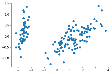
You can also plot variables in the new axis system. However, you have to use a loop to do this, because the plt.arrow function only draws one arrow at a time
PC1 = acp.components_[0]
PC2 = acp.components_[1]

for i in range(len(PC1)):
  plt.arrow(0, 0, PC1[i], PC2[i], head_width = 0.05)
  plt.text(PC1[i], PC2[i],list(donnees_pour_acp)[i])
plt.axvline(0, linestyle = "--")
plt.axhline(0, linestyle = "--")
plt.xlim(-1.5,1.5)
plt.ylim(-1,1)
(-1.0, 1.0)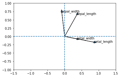
As this is not a statistics workshop, I leave you the pleasure of scaling the two data (eigenvectors and points) in the same graph with the scaling of your choice ;-)
Resources
Here are two resources that have been useful to me in building this workshop:
If you really want to learn Python, the most recommended book right now is Python Crash Course, 2nd edition, by Eric Matthes. Beyond the first 200 pages teaching you the basics of Python, the other 300 are devoted to 3 projects showing you the different facets of the language: a game including a visual interface, a data analysis project and a Web application.
If you ever want to apply what you have seen in your statistics courses with Python (and for each piece of code see the equivalent in R), I recommend Practical Statistics for Data Scientists, Second Edition, by Bruce, Bruce and Gedeck. It is both one of the few books presenting examples in two languages and it offers, in my opinion, just the right level of detail for someone who wants to apply good statistical techniques correctly, without having the ambition to become a full-time statistician.