Fast data manipulation with dplyr and its allies
Charles Martin
October 2018
- Our dataset
- The 5 base operations on a dataset
- This workshop was prepared with…
Our dataset
As in the previous workshop, we’ll use the mammal sleep dataset from ggplot2 to run our examples :
library(ggplot2)
data(msleep)
msleep
# A tibble: 83 x 11
   name   genus vore  order conservation sleep_total sleep_rem sleep_cycle
   <chr>  <chr> <chr> <chr> <chr>              <dbl>     <dbl>       <dbl>
 1 Cheet… Acin… carni Carn… lc                  12.1      NA        NA
 2 Owl m… Aotus omni  Prim… <NA>                17         1.8      NA
 3 Mount… Aplo… herbi Rode… nt                  14.4       2.4      NA
 4 Great… Blar… omni  Sori… lc                  14.9       2.3       0.133
 5 Cow    Bos   herbi Arti… domesticated         4         0.7       0.667
 6 Three… Brad… herbi Pilo… <NA>                14.4       2.2       0.767
 7 North… Call… carni Carn… vu                   8.7       1.4       0.383
 8 Vespe… Calo… <NA>  Rode… <NA>                 7        NA        NA
 9 Dog    Canis carni Carn… domesticated        10.1       2.9       0.333
10 Roe d… Capr… herbi Arti… lc                   3        NA        NA
# ... with 73 more rows, and 3 more variables: awake <dbl>, brainwt <dbl>,
#   bodywt <dbl>
The 5 base operations on a dataset
Just as in the previous workshop, all operations shown here could be done in base R. But, as you’ll see, the dplyr-way is much more integrated and easier to read (more on this later)
Filtering a dataset
For example, let’s say that you want to keep only mammals of at least 200 g
library(dplyr)
Attaching package: 'dplyr'
The following objects are masked from 'package:stats':

    filter, lag
The following objects are masked from 'package:base':

    intersect, setdiff, setequal, union
filter(msleep, bodywt > 0.2)
# A tibble: 61 x 11
   name   genus vore  order conservation sleep_total sleep_rem sleep_cycle
   <chr>  <chr> <chr> <chr> <chr>              <dbl>     <dbl>       <dbl>
 1 Cheet… Acin… carni Carn… lc                  12.1      NA        NA
 2 Owl m… Aotus omni  Prim… <NA>                17         1.8      NA
 3 Mount… Aplo… herbi Rode… nt                  14.4       2.4      NA
 4 Cow    Bos   herbi Arti… domesticated         4         0.7       0.667
 5 Three… Brad… herbi Pilo… <NA>                14.4       2.2       0.767
 6 North… Call… carni Carn… vu                   8.7       1.4       0.383
 7 Dog    Canis carni Carn… domesticated        10.1       2.9       0.333
 8 Roe d… Capr… herbi Arti… lc                   3        NA        NA
 9 Goat   Capri herbi Arti… lc                   5.3       0.6      NA
10 Guine… Cavis herbi Rode… domesticated         9.4       0.8       0.217
# ... with 51 more rows, and 3 more variables: awake <dbl>, brainwt <dbl>,
#   bodywt <dbl>
Please note that as in all object manipulations in R, the original object is not afffected and the result is “loss” unless it is assigned to a new object…
big_mammals <- filter(msleep, bodywt > 0.2)
In RStudio, you can also inspect the result of such an operation, with or without saving it first through the View function :
View(filter(msleep, bodywt > 0.2))
View(grands_mams)
Four important caveats when filtering datasets
#1 Floating point numbers are not indefinitely precise
1/49*49 == 1
[1] FALSE
This happens because when doing calculations, R can only keep a certain number of decimal places. Which means that in some cases, rounding errors can complicate comparisons.
To work around this problem, one can use the near function
near(1/49*49, 1)
[1] TRUE
#2 = doesn’t mean equal
In R, as in most programming languages, the = is used to assign the result of an operation to an object (in R, it is a synonym of <-). To check if two objects are equal, one must use the == operator.
filter(msleep, vore = "omni")
Error: `vore` (`vore = "omni"`) must not be named, do you need `==`?
3 Missing data have some unintuitive behaviors
You cannot check for missing values with the == operator
NA == NA
[1] NA
The underlying logic here being that, if I do not know Paul’s age, and I do not now Jack’s age, the answer to the question : Do Paul and Jack have the same age isn’t TRUE, it is I don’t know (NA)
To check for missing values, one must use the ia.na function :
filter(msleep, is.na(conservation))
# A tibble: 29 x 11
   name   genus vore  order conservation sleep_total sleep_rem sleep_cycle
   <chr>  <chr> <chr> <chr> <chr>              <dbl>     <dbl>       <dbl>
 1 Owl m… Aotus omni  Prim… <NA>                17         1.8      NA
 2 Three… Brad… herbi Pilo… <NA>                14.4       2.2       0.767
 3 Vespe… Calo… <NA>  Rode… <NA>                 7        NA        NA
 4 Afric… Cric… omni  Rode… <NA>                 8.3       2        NA
 5 Weste… Euta… herbi Rode… <NA>                14.9      NA        NA
 6 Galago Gala… omni  Prim… <NA>                 9.8       1.1       0.55
 7 Human  Homo  omni  Prim… <NA>                 8         1.9       1.5
 8 Macaq… Maca… omni  Prim… <NA>                10.1       1.2       0.75
 9 "Vole… Micr… herbi Rode… <NA>                12.8      NA        NA
10 Littl… Myot… inse… Chir… <NA>                19.9       2         0.2
# ... with 19 more rows, and 3 more variables: awake <dbl>, brainwt <dbl>,
#   bodywt <dbl>
#4 To combine comparisons, you need to think more like a machine
R includes operators that allow you to combine conditions either with OR (|) or AND (&). Their usage is a bit different than your normal flow of thought.
For example, if you want all mammals that are either omnivorous or carnivorous, you’d be tempted to write :
filter(msleep, vore == "omni" | "carni")
Error in filter_impl(.data, quo): Evaluation error: operations are possible only for numeric, logical or complex types.
But R is a bit dumber than that. You need to speficify every condition in details, e.g. :
filter(msleep, vore == "omni" | vore == "carni")
# A tibble: 39 x 11
   name   genus vore  order conservation sleep_total sleep_rem sleep_cycle
   <chr>  <chr> <chr> <chr> <chr>              <dbl>     <dbl>       <dbl>
 1 Cheet… Acin… carni Carn… lc                  12.1      NA        NA
 2 Owl m… Aotus omni  Prim… <NA>                17         1.8      NA
 3 Great… Blar… omni  Sori… lc                  14.9       2.3       0.133
 4 North… Call… carni Carn… vu                   8.7       1.4       0.383
 5 Dog    Canis carni Carn… domesticated        10.1       2.9       0.333
 6 Grivet Cerc… omni  Prim… lc                  10         0.7      NA
 7 Star-… Cond… omni  Sori… lc                  10.3       2.2      NA
 8 Afric… Cric… omni  Rode… <NA>                 8.3       2        NA
 9 Lesse… Cryp… omni  Sori… lc                   9.1       1.4       0.15
10 Long-… Dasy… carni Cing… lc                  17.4       3.1       0.383
# ... with 29 more rows, and 3 more variables: awake <dbl>, brainwt <dbl>,
#   bodywt <dbl>
Such a redundant syntax can easily be shortened with the %in% operator.
filter(msleep, vore %in% c("omni", "carni"))
# A tibble: 39 x 11
   name   genus vore  order conservation sleep_total sleep_rem sleep_cycle
   <chr>  <chr> <chr> <chr> <chr>              <dbl>     <dbl>       <dbl>
 1 Cheet… Acin… carni Carn… lc                  12.1      NA        NA
 2 Owl m… Aotus omni  Prim… <NA>                17         1.8      NA
 3 Great… Blar… omni  Sori… lc                  14.9       2.3       0.133
 4 North… Call… carni Carn… vu                   8.7       1.4       0.383
 5 Dog    Canis carni Carn… domesticated        10.1       2.9       0.333
 6 Grivet Cerc… omni  Prim… lc                  10         0.7      NA
 7 Star-… Cond… omni  Sori… lc                  10.3       2.2      NA
 8 Afric… Cric… omni  Rode… <NA>                 8.3       2        NA
 9 Lesse… Cryp… omni  Sori… lc                   9.1       1.4       0.15
10 Long-… Dasy… carni Cing… lc                  17.4       3.1       0.383
# ... with 29 more rows, and 3 more variables: awake <dbl>, brainwt <dbl>,
#   bodywt <dbl>
The %in% can also be used to list you prepare before your statement…
to_keep <- c("omni", "carni", "herbi")
filter(msleep, vore %in% to_keep)
# A tibble: 71 x 11
   name   genus vore  order conservation sleep_total sleep_rem sleep_cycle
   <chr>  <chr> <chr> <chr> <chr>              <dbl>     <dbl>       <dbl>
 1 Cheet… Acin… carni Carn… lc                  12.1      NA        NA
 2 Owl m… Aotus omni  Prim… <NA>                17         1.8      NA
 3 Mount… Aplo… herbi Rode… nt                  14.4       2.4      NA
 4 Great… Blar… omni  Sori… lc                  14.9       2.3       0.133
 5 Cow    Bos   herbi Arti… domesticated         4         0.7       0.667
 6 Three… Brad… herbi Pilo… <NA>                14.4       2.2       0.767
 7 North… Call… carni Carn… vu                   8.7       1.4       0.383
 8 Dog    Canis carni Carn… domesticated        10.1       2.9       0.333
 9 Roe d… Capr… herbi Arti… lc                   3        NA        NA
10 Goat   Capri herbi Arti… lc                   5.3       0.6      NA
# ... with 61 more rows, and 3 more variables: awake <dbl>, brainwt <dbl>,
#   bodywt <dbl>
Conditions can also be reversed
The exclamations point(!) can be used to inverse the result of a condition. For example, to extract all mammals except for omnivorous ones :
filter(msleep, !(vore == "omni"))
# A tibble: 56 x 11
   name   genus vore  order conservation sleep_total sleep_rem sleep_cycle
   <chr>  <chr> <chr> <chr> <chr>              <dbl>     <dbl>       <dbl>
 1 Cheet… Acin… carni Carn… lc                  12.1      NA        NA
 2 Mount… Aplo… herbi Rode… nt                  14.4       2.4      NA
 3 Cow    Bos   herbi Arti… domesticated         4         0.7       0.667
 4 Three… Brad… herbi Pilo… <NA>                14.4       2.2       0.767
 5 North… Call… carni Carn… vu                   8.7       1.4       0.383
 6 Dog    Canis carni Carn… domesticated        10.1       2.9       0.333
 7 Roe d… Capr… herbi Arti… lc                   3        NA        NA
 8 Goat   Capri herbi Arti… lc                   5.3       0.6      NA
 9 Guine… Cavis herbi Rode… domesticated         9.4       0.8       0.217
10 Chinc… Chin… herbi Rode… domesticated        12.5       1.5       0.117
# ... with 46 more rows, and 3 more variables: awake <dbl>, brainwt <dbl>,
#   bodywt <dbl>
Sorting
By default, sorting in R happens in an ascending way
arrange(msleep, bodywt)
# A tibble: 83 x 11
   name   genus vore  order conservation sleep_total sleep_rem sleep_cycle
   <chr>  <chr> <chr> <chr> <chr>              <dbl>     <dbl>       <dbl>
 1 Lesse… Cryp… omni  Sori… lc                   9.1       1.4       0.15
 2 Littl… Myot… inse… Chir… <NA>                19.9       2         0.2
 3 Great… Blar… omni  Sori… lc                  14.9       2.3       0.133
 4 Deer … Pero… <NA>  Rode… <NA>                11.5      NA        NA
 5 House… Mus   herbi Rode… nt                  12.5       1.4       0.183
 6 Big b… Epte… inse… Chir… lc                  19.7       3.9       0.117
 7 North… Onyc… carni Rode… lc                  14.5      NA        NA
 8 "Vole… Micr… herbi Rode… <NA>                12.8      NA        NA
 9 Afric… Rhab… omni  Rode… <NA>                 8.7      NA        NA
10 Vespe… Calo… <NA>  Rode… <NA>                 7        NA        NA
# ... with 73 more rows, and 3 more variables: awake <dbl>, brainwt <dbl>,
#   bodywt <dbl>
You need to add a special modifier to reverse that order
arrange(msleep, desc(bodywt))
# A tibble: 83 x 11
   name   genus vore  order conservation sleep_total sleep_rem sleep_cycle
   <chr>  <chr> <chr> <chr> <chr>              <dbl>     <dbl>       <dbl>
 1 Afric… Loxo… herbi Prob… vu                   3.3      NA        NA
 2 Asian… Elep… herbi Prob… en                   3.9      NA        NA
 3 Giraf… Gira… herbi Arti… cd                   1.9       0.4      NA
 4 Pilot… Glob… carni Ceta… cd                   2.7       0.1      NA
 5 Cow    Bos   herbi Arti… domesticated         4         0.7       0.667
 6 Horse  Equus herbi Peri… domesticated         2.9       0.6       1
 7 Brazi… Tapi… herbi Peri… vu                   4.4       1         0.9
 8 Donkey Equus herbi Peri… domesticated         3.1       0.4      NA
 9 Bottl… Turs… carni Ceta… <NA>                 5.2      NA        NA
10 Tiger  Pant… carni Carn… en                  15.8      NA        NA
# ... with 73 more rows, and 3 more variables: awake <dbl>, brainwt <dbl>,
#   bodywt <dbl>
Exercise one
Find, in ascending order of body weight, the list of all non-domestic herbivorous animals
Select some columns
select(msleep, vore, brainwt, bodywt)
# A tibble: 83 x 3
   vore   brainwt  bodywt
   <chr>    <dbl>   <dbl>
 1 carni NA        50
 2 omni   0.0155    0.48
 3 herbi NA         1.35
 4 omni   0.00029   0.019
 5 herbi  0.423   600
 6 herbi NA         3.85
 7 carni NA        20.5
 8 <NA>  NA         0.045
 9 carni  0.07     14
10 herbi  0.0982   14.8
# ... with 73 more rows
You can also specify a series of columns, as long as they are adjacent in the dataset
select(msleep, sleep_total:awake)
# A tibble: 83 x 4
   sleep_total sleep_rem sleep_cycle awake
         <dbl>     <dbl>       <dbl> <dbl>
 1        12.1      NA        NA      11.9
 2        17         1.8      NA       7
 3        14.4       2.4      NA       9.6
 4        14.9       2.3       0.133   9.1
 5         4         0.7       0.667  20
 6        14.4       2.2       0.767   9.6
 7         8.7       1.4       0.383  15.3
 8         7        NA        NA      17
 9        10.1       2.9       0.333  13.9
10         3        NA        NA      21
# ... with 73 more rows
Please note that, as before, as long as you don’t override the object, the original dataset is not affected by column selection.
Adding columns
Because columns are added (by default) to the rightmost of the dataset, we create ourselves a simplified dataset just to see more easily what we are doing.
weights <- select(msleep,ends_with("wt"))
weights
# A tibble: 83 x 2
    brainwt  bodywt
      <dbl>   <dbl>
 1 NA        50
 2  0.0155    0.48
 3 NA         1.35
 4  0.00029   0.019
 5  0.423   600
 6 NA         3.85
 7 NA        20.5
 8 NA         0.045
 9  0.07     14
10  0.0982   14.8
# ... with 73 more rows
To add a column containing brain size in grams instead of kilograms
mutate(weights, cerveau_g = brainwt*1000)
# A tibble: 83 x 3
    brainwt  bodywt cerveau_g
      <dbl>   <dbl>     <dbl>
 1 NA        50        NA
 2  0.0155    0.48     15.5
 3 NA         1.35     NA
 4  0.00029   0.019     0.290
 5  0.423   600       423
 6 NA         3.85     NA
 7 NA        20.5      NA
 8 NA         0.045    NA
 9  0.07     14        70
10  0.0982   14.8      98.2
# ... with 73 more rows
Note that many columns can be used in the same calculation, e.g. to calculate the relative size of the brain :
mutate(weights, rel_brain = brainwt / bodywt)
# A tibble: 83 x 3
    brainwt  bodywt rel_brain
      <dbl>   <dbl>     <dbl>
 1 NA        50     NA
 2  0.0155    0.48   0.0323
 3 NA         1.35  NA
 4  0.00029   0.019  0.0153
 5  0.423   600      0.000705
 6 NA         3.85  NA
 7 NA        20.5   NA
 8 NA         0.045 NA
 9  0.07     14      0.005
10  0.0982   14.8    0.00664
# ... with 73 more rows
Combining many operations in a chain
This is where, in my opinion, that the dplyr-way really shines.
With the few functions we’ve seen so far, we can already do a lot of things. For example, if we wished to find the name and the weight of the 10 smallest mammals in the dataset :
x <- arrange(msleep,bodywt) # sort from smallest to largest
y <- mutate(x,rang = row_number())# add a rank column
z <- filter(y, rang <= 10)# keep only the 10 smallest ones
select(z,name,bodywt)# keep only name and weight columns
# A tibble: 10 x 2
   name                       bodywt
   <chr>                       <dbl>
 1 Lesser short-tailed shrew   0.005
 2 Little brown bat            0.01
 3 Greater short-tailed shrew  0.019
 4 Deer mouse                  0.021
 5 House mouse                 0.022
 6 Big brown bat               0.023
 7 Northern grasshopper mouse  0.028
 8 "Vole "                     0.035
 9 African striped mouse       0.044
10 Vesper mouse                0.045
Notice that on the way, we create many useless intermediate objects (x,y and z), which we could easily eliminate.
select(filter(mutate(arrange(msleep,bodywt),rang = row_number()), rang <= 10),name,bodywt)
But doing so, we loose a lot in readability. We could split that code again into separate lines and use identation to clarify things :
select(
  filter(
    mutate(
      arrange(msleep,bodywt),
      rang = row_number()
    ),
    rang <= 10
  ),
  name,
  bodywt
)
But the resulting code is not necessarily easy to read, and at first sight, it’s hard to know which dataset is affected. It is also annoying that you need to read from center to the outside, which is not natural for most readers.
This is where the pipe operator (%>%) from the magrittr library comes in really handy :
msleep %>%
  arrange(bodywt) %>%
  mutate(rang = row_number()) %>%
  filter(rang <= 10) %>%
  select(name, bodywt)
NB there is no need to manually load the pipe operator as dplyr does this for us everytime we load it.
%>% transforms our code in a way that is easier for us, while keeping it interpretable by R…
- Code becomes easier to read
- We get back our natural left-to-right and top-to-bottom reading sequence
- No more intermediate objects littering our code
- The dataset is the first thing in the chain, clearly indicating on what the code applies
- Every line of code begins with an action verb
I know, %>% is clunky to type, but those of you with RStudio can use the : Ctrl+Shift+M to type it rapidly.
All librairies from Hadley Wickam’s tidyverse are required to support the pipe operator… except one : ggplot2.
ggplot2 doesn’t support the pipe operator, and probably never will. You can read the whole story here : https://community.rstudio.com/t/why-cant-ggplot2-use/4372/7.
ggplot2 can nevertheless be inserted at the end of a chain :
msleep %>%
  filter(bodywt > 0.200) %>%
  mutate(
    l_corps = log(bodywt),
    l_cerveau = log(brainwt)
  ) %>%
  ggplot(aes(x = l_corps,y = l_cerveau, col = vore)) +
  geom_point()
Warning: Removed 19 rows containing missing values (geom_point).
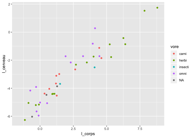
Mixing ggplot2 with dplyr forces you to be very alert, because you now have database manipulation statements chained together with %>% a graphic layers connected with +
Second exercise
Just try again the first exercise (finding, in ascending order of body weight, the list of all non-domestic herbivorous animals) but this time, taking advantage of the pipe operator to simplify your code.
Summarizing a dataset
With the summarize function, you can summarize many functions or variables at once :
msleep %>%
  summarize(
    mean_weight = mean(bodywt),
    sd_weight = sd(bodywt)
  )
# A tibble: 1 x 2
  mean_weight sd_weight
        <dbl>            <dbl>
1        166.             787.
Such an operation becomes much more powerful if we use a grouping clause :
msleep %>%
  group_by(vore) %>%
  summarize(
    mean_weight = mean(bodywt),
    sd_weight = sd(bodywt)
  )
# A tibble: 5 x 3
  vore    mean_weidth        sd_weight
  <chr>         <dbl>            <dbl>
1 carni        90.8             182.
2 herbi       367.             1244.
3 insecti      12.9              26.4
4 omni         12.7              24.7
5 <NA>          0.858             1.34
This workshop was prepared with…
sessionInfo()
R version 3.5.1 (2018-07-02)
Platform: x86_64-apple-darwin15.6.0 (64-bit)
Running under: macOS High Sierra 10.13.6

Matrix products: default
BLAS: /Library/Frameworks/R.framework/Versions/3.5/Resources/lib/libRblas.0.dylib
LAPACK: /Library/Frameworks/R.framework/Versions/3.5/Resources/lib/libRlapack.dylib

locale:
[1] en_US.UTF-8/en_US.UTF-8/en_US.UTF-8/C/en_US.UTF-8/en_US.UTF-8

attached base packages:
[1] stats     graphics  grDevices utils     datasets  methods   base

other attached packages:
[1] readxl_1.1.0   tidyr_0.8.1    bindrcpp_0.2.2 dplyr_0.7.7
[5] ggplot2_3.0.0

loaded via a namespace (and not attached):
 [1] Rcpp_0.12.17     pillar_1.2.3     compiler_3.5.1   cellranger_1.1.0
 [5] plyr_1.8.4       bindr_0.1.1      tools_3.5.1      digest_0.6.15
 [9] evaluate_0.10.1  tibble_1.4.2     gtable_0.2.0     pkgconfig_2.0.1
[13] rlang_0.2.1      cli_1.0.0        yaml_2.1.19      withr_2.1.2
[17] stringr_1.3.1    knitr_1.20       rprojroot_1.3-2  grid_3.5.1
[21] tidyselect_0.2.4 glue_1.2.0       R6_2.2.2         rmarkdown_1.10
[25] purrr_0.2.5      magrittr_1.5     backports_1.1.2  scales_0.5.0
[29] htmltools_0.3.6  assertthat_0.2.0 colorspace_1.3-2 labeling_0.3
[33] utf8_1.1.4       stringi_1.2.3    lazyeval_0.2.1   munsell_0.5.0
[37] crayon_1.3.4