Time Series with MARSS
Lucas Deschamps & Isabelle Gosselin
May 2021
- Introduction
- Dataset
- Decomposition of the time series
- Modelling
- Intercept only model
- Quantification of predictive accuracy
- Conclusion
Introduction
The classic statistical framework hardly applies to time-series, partly because they are unique. Conversely to experiments, for example, one cannot replicate time-series : we cannot replicate the size of the human population from Trois-Rivieres, or the St-Maurice throughput, we can only measure them regularly.
Very often, time-series analysis has concrete predictive applications. One may seek to predict the future price of a product, or to interpolate the value of a fish population at a year during which no measurement was realized.
The world of time-series analysis is extremely complex, with its own jargon. One can model time dependency using, among many others,
- gaussian processes (an option I like and currently use), implemented in the
brmsandmgcvpackage; - splines, as implemented in
rstanarm,brmsandmgcv; - Differential equations, which can be fitted using
stanand are heavily used in physics and pharmacometry, for example. - ARIMA, as implemented in
ARIMA.
We will focus on a state-space approach, which has solid theoretical foundation which allow to make inferences in a way close to the foundation and ecological and system sciences (see for example a classical Markov process describing a succession toward a climax)
The resources we used to build the present workshop are
https://nwfsc-timeseries.github.io/
A very complete website from the creators of the MARSS package, including a web-based book, many recorded courses with slides packages resources.
https://otexts.com/fpp2/data-methods.html
An introduction to forecasting using ARIMA and dlm approaches, very complete.
https://cran.r-project.org/web/packages/MARSS/vignettes/UserGuide.pdf
The user guide of the MARSS package.
Dataset
The dataset we will use contains the abundances of many phytoplanktonic and zooplanktonic taxa, measured in the Lake Washington from 1962 to 1994, with three covariates (pH, Dissolved Oxygen and Temperature). All variables are logged and scaled.
library(MARSS)

data(lakeWAplankton, package = "MARSS")

D <- lakeWAplanktonTrans
str(D)
##  num [1:396, 1:20] 1962 1962 1962 1962 1962 ...
##  - attr(*, "dimnames")=List of 2
##   ..$ : NULL
##   ..$ : chr [1:20] "Year" "Month" "Temp" "TP" ...
summary(D)
##       Year          Month            Temp                 TP
##  Min.   :1962   Min.   : 1.00   Min.   :-1.844659   Min.   :-0.990384
##  1st Qu.:1970   1st Qu.: 3.75   1st Qu.:-0.986030   1st Qu.:-0.587223
##  Median :1978   Median : 6.50   Median :-0.039857   Median :-0.348895
##  Mean   :1978   Mean   : 6.50   Mean   :-0.002465   Mean   : 0.013290
##  3rd Qu.:1986   3rd Qu.: 9.25   3rd Qu.: 0.906710   3rd Qu.:-0.001897
##  Max.   :1994   Max.   :12.00   Max.   : 2.059220   Max.   : 5.606247
##
##        pH           Cryptomonas         Diatoms             Greens
##  Min.   :-2.5763   Min.   :-4.6075   Min.   :-2.56501   Min.   :-3.06213
##  1st Qu.:-0.7126   1st Qu.:-0.4104   1st Qu.:-0.68656   1st Qu.:-0.56478
##  Median :-0.1587   Median : 0.1755   Median :-0.07171   Median : 0.01288
##  Mean   : 0.0000   Mean   : 0.0000   Mean   : 0.00000   Mean   : 0.00000
##  3rd Qu.: 0.4963   3rd Qu.: 0.6277   3rd Qu.: 0.76881   3rd Qu.: 0.55290
##  Max.   : 3.7536   Max.   : 2.1342   Max.   : 2.65264   Max.   : 3.26256
##  NA's   :2         NA's   :122       NA's   :3          NA's   :40
##    Bluegreens         Unicells         Other.algae         Conochilus
##  Min.   :-3.0834   Min.   :-4.32401   Min.   :-2.98823   Min.   :-2.24700
##  1st Qu.:-0.4832   1st Qu.:-0.66333   1st Qu.:-0.70038   1st Qu.:-0.76468
##  Median : 0.2733   Median :-0.02512   Median : 0.01709   Median : 0.08651
##  Mean   : 0.0000   Mean   : 0.00000   Mean   : 0.00000   Mean   : 0.00000
##  3rd Qu.: 0.7334   3rd Qu.: 0.72201   3rd Qu.: 0.71167   3rd Qu.: 0.78488
##  Max.   : 1.3534   Max.   : 2.65662   Max.   : 2.51383   Max.   : 2.23467
##  NA's   :185       NA's   :3          NA's   :4          NA's   :90
##     Cyclops            Daphnia          Diaptomus          Epischura
##  Min.   :-2.65924   Min.   :-2.7218   Min.   :-2.76122   Min.   :-4.50267
##  1st Qu.:-0.61934   1st Qu.:-0.7752   1st Qu.:-0.67663   1st Qu.:-0.58893
##  Median : 0.04852   Median : 0.2320   Median :-0.01564   Median : 0.08079
##  Mean   : 0.00000   Mean   : 0.0000   Mean   : 0.00000   Mean   : 0.00000
##  3rd Qu.: 0.66758   3rd Qu.: 0.8792   3rd Qu.: 0.71827   3rd Qu.: 0.72851
##  Max.   : 2.72409   Max.   : 1.6079   Max.   : 2.38983   Max.   : 2.08288
##  NA's   :8          NA's   :125       NA's   :8          NA's   :10
##    Leptodora           Neomysis       Non.daphnid.cladocerans
##  Min.   :-2.22557   Min.   :-1.3091   Min.   :-3.4867
##  1st Qu.:-0.71551   1st Qu.:-0.6481   1st Qu.:-0.5884
##  Median : 0.07669   Median :-0.1740   Median : 0.1023
##  Mean   : 0.00000   Mean   : 0.0000   Mean   : 0.0000
##  3rd Qu.: 0.67685   3rd Qu.: 0.5553   3rd Qu.: 0.7374
##  Max.   : 2.08438   Max.   : 3.2076   Max.   : 2.1074
##  NA's   :207        NA's   :348       NA's   :11
##  Non.colonial.rotifers
##  Min.   :-2.61920
##  1st Qu.:-0.66585
##  Median :-0.02207
##  Mean   : 0.00000
##  3rd Qu.: 0.68769
##  Max.   : 2.97901
##  NA's   :8
To make plots and patterns clearer, we will only select a 10 years long duration. We will keep the last year unused to check our predictions later.
yr_frst <- 1980
yr_last <- 1989
# Filtrer entre yr_frst et yr_last
Plank <- D[D[, "Year"] >= yr_frst & D[,
    "Year"] <= yr_last, ]
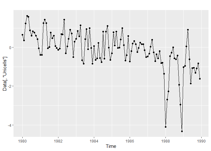
For this workshop, we will only focus on Unicells algae dynamic. A lot of R function allowing to visualize and analyze time-series need to be fed with a ts objects (from stats), which we create with the following code. We use the first row of the data set to specify the starting dates of the time series, and because we use monthly measured data, we specify frequency = 12.
We need the forecast package to make nice gg-based plots of ts objects.
Data <- ts(Plank[, c("Year", "Month", "Unicells")], frequency = 12,
           start = c(Plank[1, "Year"], Plank[1, "Month"]))

library(forecast)
library(ggplot2)
autoplot(Data[,"Unicells"]) +
  geom_point()
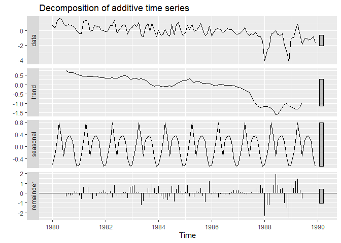
Decomposition of the time series
Time-series may be composed of four abstract elements :
- a trend;
- a seasonality. For example, each data measured in January may look like other data from January, each data measured a 1 AM may look like other values measured at 1 AM.
- a cyclicity. For example, the Quebec Lynx population has been demonstrated to experience regularly spaced increase and decrease, unrelated to any seasonal pattern.
- a residual noise.
decompose is a useful function to visualize these elements in a time-series. Filter used in decomposition may be parametrized depending upon our needs, but we will use the default for sake of simplicity. One can find more information here
autoplot(decompose(Data[,"Unicells"]))
Modelling
Decomposition is very interesting to have a taste about what composed our time-series, but it cannot produce statistical inferences nor predictions. To do that, we need a statistical model representing the processes which produced our data, and translate it into probabilistic equations.
The State-Space approach used in the MARSS package allow to assemble in one conceptual framework many notions gathered from different forecasting approaches. It is also closely related to system science, which is what we study as ecologist!
MARSS stands for Multivariate Autoregressive State-Space modeling. We will only gently scratch the surface of what can be done with this package, by using only a univariate time-series and parameters fixed in time.
Functions from this package need time to go across columns, so we will transpose our data set.
Datat <- t(Data)
MARSS model structure
In a State-Space model, the value of the y variable a time t is the result of a latent process, represented by x, plus a random noise. The name of the different parameters are important to remember, because we will specify how we want to estimate them.
# y_t = Z * x_t + a + v_t
# v_t ~ normal(0,R)
- We wont use
Zanda, they are destined to more complex multivariate model we won’t approach. v_tcorrespond to a gaussian noise parametrized by its standard-deviationRx_tis the value of the underlying process at timet, which depends upon the precente value of the process.
# x_t = B * x_(t-1) + u + w_t
# w_t ~ normal(0,Q)
Bmultiplies the previous state value, and will allow to model an auto-regressive process.ucorresponds to a drift. If the value at timetis equal to the value at timet-1more or less a constant, this will create a tendency.w_tcorresponds to a random-walk modification added to the precedent states. It is a gaussian processual noise of standard-deviationQ.
The initial states, x0 is also necessary to estimate in the problem we are interested in!
# x_0 = mu
Intercept only model
We will fix every parameters except mu and R
- B = 1 (no auto-regression)
- u = 0 (no drift)
- Q = 0 (no random-walk)
- Z = 1
- a = 0
- we estimate mu (initial latent-state)
- we estimate R (noise aroung the latent state)
Because the program uses linear algebra in its optimization approach, we have to provide the parameters as matrices. Fixed parameters are inputed with number, while estimated ones with letters.
mod.list.int <- list(B = matrix(1), U = matrix(0), Q = matrix(0),
                     Z = matrix(1), A = matrix(0), R = matrix("sd_obs"),
                     x0 = matrix("init.state"))
Let’s fit the model! The default convergence settings are slightly louss, we can tighten it as suggested by added the commented par of the code inside the function.
fit.int <- MARSS(Datat["Unicells",], model = mod.list.int)
## Success! algorithm run for 15 iterations. abstol and log-log tests passed.
## Alert: conv.test.slope.tol is 0.5.
## Test with smaller values (<0.1) to ensure convergence.
##
## MARSS fit is
## Estimation method: kem
## Convergence test: conv.test.slope.tol = 0.5, abstol = 0.001
## Algorithm ran 15 (=minit) iterations and convergence was reached.
## Log-likelihood: -168.9704
## AIC: 341.9408   AICc: 342.0434
##
##               Estimate
## R.sd_obs         0.979
## x0.init.state   -0.115
## Initial states (x0) defined at t=0
##
## Standard errors have not been calculated.
## Use MARSSparamCIs to compute CIs and bias estimates.
# control = list(conv.test.slope.tol = 0.1))
Uncertainty around parameters is not reported, but we can obtain it simply using the following function :
MARSSparamCIs(fit.int)
##
## MARSS fit is
## Estimation method: kem
## Convergence test: conv.test.slope.tol = 0.5, abstol = 0.001
## Algorithm ran 15 (=minit) iterations and convergence was reached.
## Log-likelihood: -168.9704
## AIC: 341.9408   AICc: 342.0434
##
##               ML.Est Std.Err low.CI up.CI
## R.sd_obs       0.979  0.1263  0.731 1.226
## x0.init.state -0.115  0.0903 -0.292 0.062
## Initial states (x0) defined at t=0
##
## CIs calculated at alpha = 0.05 via method=hessian
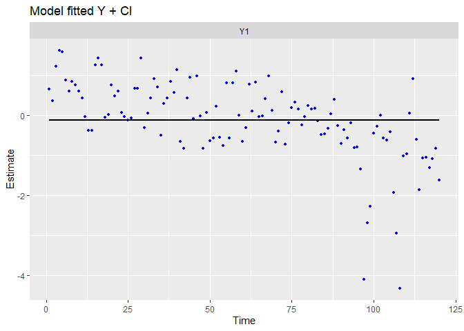
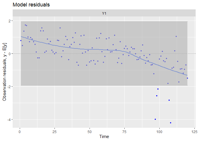
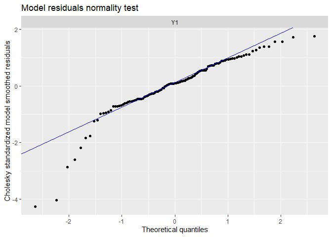
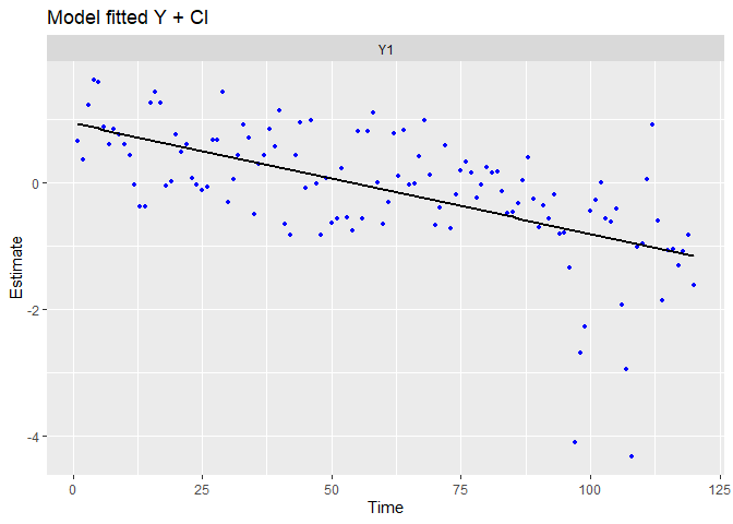
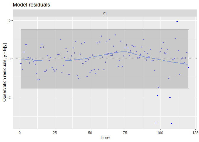
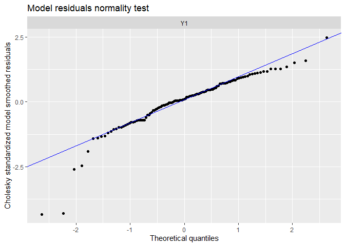
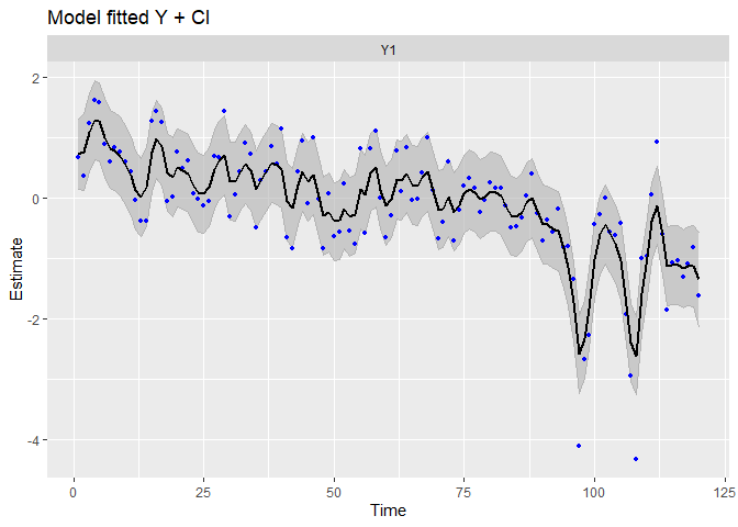
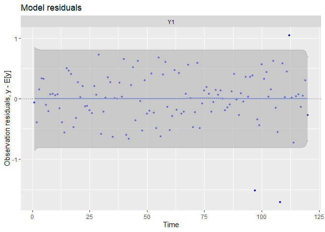
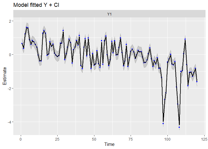
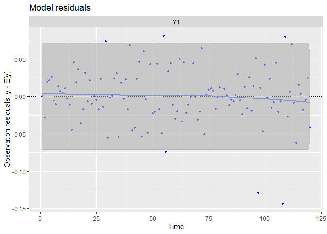
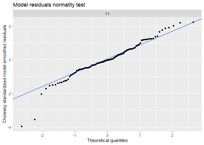
When used on the fit object, the autoplot function provides a very interesting set of plots allowing to evaluate the fit and the assumption of the model. For now, we will use three plots :
- The fitted values during time-series (in-sample predictions),
- Time dynamic of residuals,
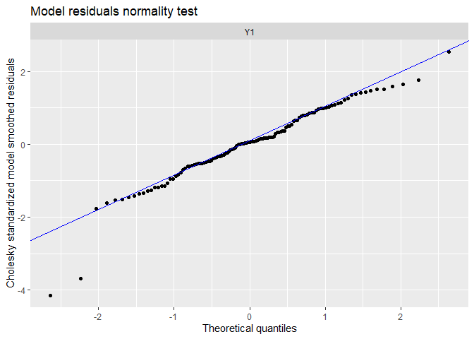
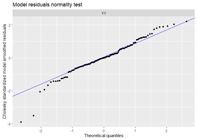
- Correspondance between the distribution of the residuals and a normal distribution
Just to be sure, the residuals are the vertical distances between each data points and the fitted value.
autoplot(fit.int, plot.type = c("model.ytT", "model.resids", "qqplot.model.resids"))
## plot.type = model.ytT
## Hit <Return> to see next plot (q to exit):
## plot.type = model.resids
## Hit <Return> to see next plot (q to exit):
## plot.type = qqplot.model.resids
## Finished plots.
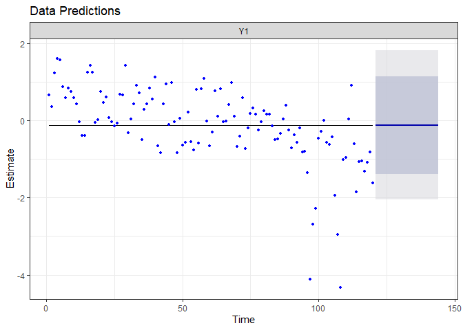
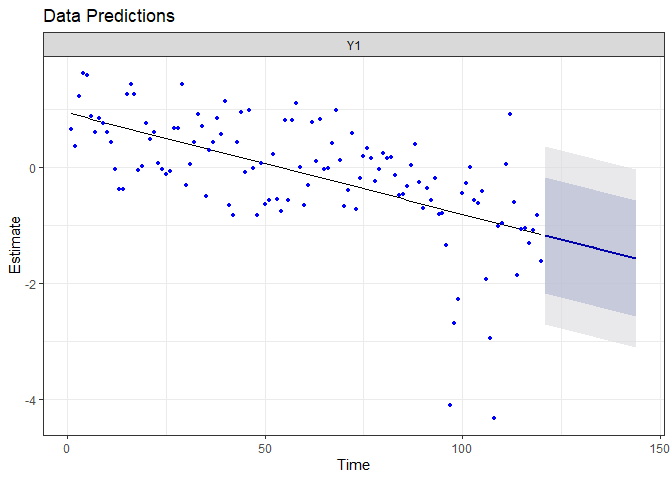
The fitted values lies on an horizontal straight line, as specified (model contains only an intercept and some observational noise).
There is a strong trends in the residuals, suggesting we did not capture accurately time dynamic with this simple model.
The tails of the qq-plots does not lie on the straight line, suggesting we observe extreme deviations to the fit not expected by a normal distribution.
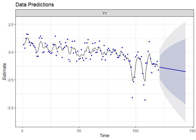
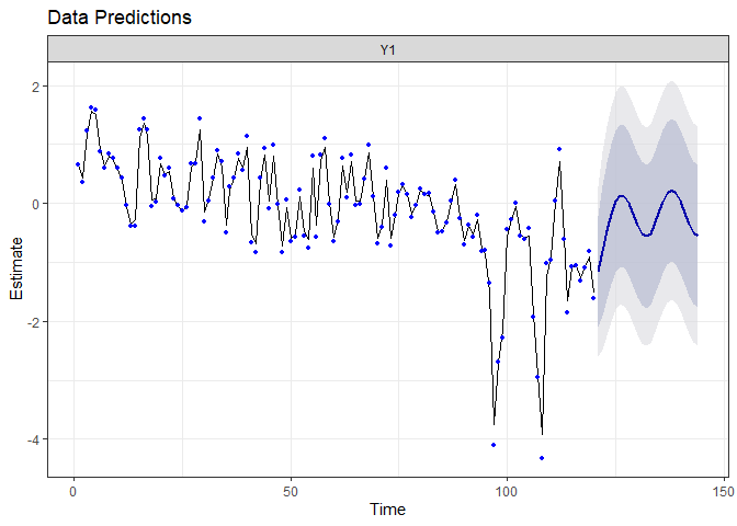
Now, let’s forecast! We will compute predicted value for two years (24 months after the end of the time-series). To obtain the latent-states value, the forecast function will use a Kalman filter. We won’t explain it, but it is important in many models and application, you can read more about it here.
fr.int <- forecast.marssMLE(fit.int, h = 24)
The autoplot function, applied to a forecast object, provide a fancy graph quickly.
autoplot(fr.int)
Drift model
We will now free the u parameter
- B = 1 (no auto-regression)
- we estimate u, the drift parameter
- Q = 0 (no random-walk)
- Z = 1
- a = 0
- we estimate mu (initial latent-state)
- we estimate R (noise aroung the latent state)
mod.list.drift <- list(B = matrix(1), U = matrix("drift"), Q = matrix(0),
                     Z = matrix(1), A = matrix(0), R = matrix("sd_obs"),
                     x0 = matrix("init.state"))
Let’s fit the model…
fit.drift <- MARSS(Datat["Unicells",], model = mod.list.drift)
## Success! abstol and log-log tests passed at 20 iterations.
## Alert: conv.test.slope.tol is 0.5.
## Test with smaller values (<0.1) to ensure convergence.
##
## MARSS fit is
## Estimation method: kem
## Convergence test: conv.test.slope.tol = 0.5, abstol = 0.001
## Estimation converged in 20 iterations.
## Log-likelihood: -140.5706
## AIC: 287.1411   AICc: 287.348
##
##               Estimate
## R.sd_obs        0.6096
## U.drift        -0.0175
## x0.init.state   0.9395
## Initial states (x0) defined at t=0
##
## Standard errors have not been calculated.
## Use MARSSparamCIs to compute CIs and bias estimates.
# control = list(conv.test.slope.tol = 0.1))
And evaluate it.
autoplot(fit.drift, plot.type = c("model.ytT", "model.resids", "qqplot.model.resids"))
## plot.type = model.ytT
## Hit <Return> to see next plot (q to exit):
## plot.type = model.resids
## Hit <Return> to see next plot (q to exit):
## plot.type = qqplot.model.resids
## Finished plots.
The trends has been visually well capture, and there is no residual linear trends. There is still some extreme residuals.
Let’s forecast!
fr.drift <- forecast.marssMLE(fit.drift, h = 24)

autoplot(fr.drift)
Because we did not allow the model to capture more information, it expect the linear decreasing trend to persist in the next two years.
Drift + random-walk model
We will now free the noise at the process level, Q, leading to a random-walk model.
- B = 1 (no auto-regression)
- we estimate u, the drift
- we estimate Q, the standard-deviation of the random-walk
- Z = 1
- a = 0
- we estimate mu (initial latent-state)
- we estimate R (noise aroung the latent state)
mod.list.randrift <- list(B = matrix(1), U = matrix("drift"), Q = matrix("sd_proc"),
                     Z = matrix(1), A = matrix(0), R = matrix("sd_obs"),
                     x0 = matrix("init.state"))
Let’s fit the model…
fit.randrift <- MARSS(Datat["Unicells",], model = mod.list.randrift)
## Success! algorithm run for 15 iterations. abstol and log-log tests passed.
## Alert: conv.test.slope.tol is 0.5.
## Test with smaller values (<0.1) to ensure convergence.
##
## MARSS fit is
## Estimation method: kem
## Convergence test: conv.test.slope.tol = 0.5, abstol = 0.001
## Algorithm ran 15 (=minit) iterations and convergence was reached.
## Log-likelihood: -143.4352
## AIC: 294.8704   AICc: 295.2182
##
##               Estimate
## R.sd_obs        0.2796
## U.drift        -0.0174
## Q.sd_proc       0.2041
## x0.init.state   0.7432
## Initial states (x0) defined at t=0
##
## Standard errors have not been calculated.
## Use MARSSparamCIs to compute CIs and bias estimates.
# control = list(conv.test.slope.tol = 0.1))
And evaluate it.
autoplot(fit.randrift, plot.type = c("model.ytT", "model.resids", "qqplot.model.resids"))
## plot.type = model.ytT
## Hit <Return> to see next plot (q to exit):
## plot.type = model.resids
## Hit <Return> to see next plot (q to exit):
## plot.type = qqplot.model.resids
## Finished plots.
We can see patterns in the data have been captured far better!
Let’s forecast!
fr.randrift <- forecast.marssMLE(fit.randrift, h = 24)

autoplot(fr.randrift)
Even if the random-walk better captures the observed patterns, it add noise to the process equation, making the prediction far less certain (which is honest!).
Auto-regressive model
As its name suggest, the auto-correlation captures the correlation between a time-series and a lagged version of itself (“auto”). It can been visualize in multiple ways.
gglagplot(Data[,"Unicells"], lags = 4)
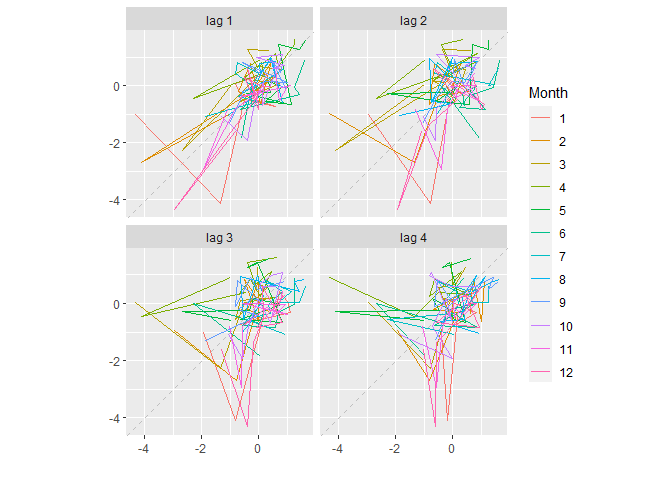
On this first graph, we can see actual values and values lagged by an order 1 lies relatively tightly on the 1:1 line, suggesting Unicells abundances at time t are strongly related to the abundances at time t-1.
An autocorrelation allows to visualize the autocorrelation (Acf) computed at different lag.
ggAcf(Data[,"Unicells"])
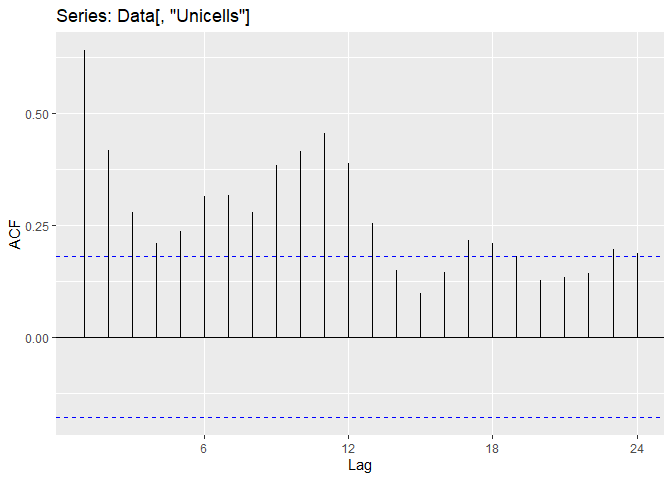
We can observe to different major auto-correlation in the Unicells abundances
- The lag(1) autocorrelation detected in the precedent plot
- A lag(~12) autocorrelation, capturing the seasonality of the data : a value at time t is similar to the value 12 month earlier.
To fit a auto-regressive model, we can free the B parameter in the process equation.
- we estimate B, the auto-regressive parameter
- we estimate u, the drift
- we estimate Q, the standard-deviation of the random-walk
- Z = 1
- a = 0
- we estimate mu (initial latent-state)
- we estimate R (noise aroung the latent state)
mod.list.auto <- list(B = matrix("autoreg"), U = matrix("drift"), Q = matrix("sd_proc"),
                     Z = matrix(1), A = matrix(0), R = matrix("sd_obs"),
                     x0 = matrix("init.state"))
Let’s fit the model. We will use the BFGS rather than the Expectation-Maximization algorithm because it is quicker and may have less convergence problems.
fit.auto <- MARSS(Datat["Unicells",], model = mod.list.auto,
                  method = "BFGS")
## Success! Converged in 79 iterations.
## Function MARSSkfas used for likelihood calculation.
##
## MARSS fit is
## Estimation method: BFGS
## Estimation converged in 79 iterations.
## Log-likelihood: -136.097
## AIC: 282.194   AICc: 282.7203
##
##               Estimate
## R.sd_obs        0.0230
## B.autoreg       0.6674
## U.drift        -0.0529
## Q.sd_proc       0.5330
## x0.init.state   1.0668
## Initial states (x0) defined at t=0
##
## Standard errors have not been calculated.
## Use MARSSparamCIs to compute CIs and bias estimates.
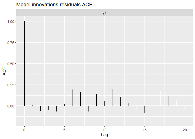
Now we are familiar with the Acf plot, so we will also observe the auto-correlation of the residuals!
autoplot(fit.auto, plot.type = c("model.ytT", "model.resids", "qqplot.model.resids", "acf.model.resids"))
## plot.type = model.ytT
## Hit <Return> to see next plot (q to exit):
## plot.type = model.resids
## Hit <Return> to see next plot (q to exit):
## plot.type = qqplot.model.resids
## Hit <Return> to see next plot (q to exit):

## plot.type = acf.model.resids
## Finished plots.
We can see the data have been very well (too well?) reproduced, and there is almost no tendency neither auto-correlation remaining in residuals. We can compare with the precedent random-walk model.
autoplot(fit.randrift, plot.type = c("acf.model.resids"))
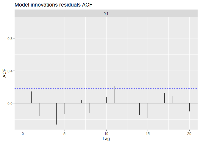 We can see the precedent model remove a lot of auto-correlation, but produced negative autocorrelation around a 3-4 month lag.
Let’s forecast!
fr.auto <- forecast.marssMLE(fit.auto, h = 24)

autoplot(fr.auto)
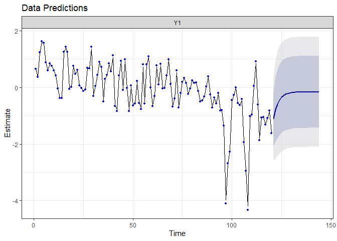
The prediction for the next two years are really different from the precedent model. Because the auto-regressive parameter is constant and deterministic, the interval of the prediction is reduced compared to the random-walk model. However, the auto-regressive model suggest the drift will not continue any further : it expects the system to return quickly to its mean value! We will check a little bit latter if this prediction is confirmed.
Seasonality
To model seasonality, we will a a covariate to the model, c_t, and expand the process-level equation by adding a “slope”, C.
# x_t = B * x_(t-1) + C * c_t + u + w_t
# w_t ~ normal(0,Q)
C_t is a matrix containing the value of the covariates at time t.
To capture seasonality, we will create a new variable representing the periodic similarity between the months of different years.
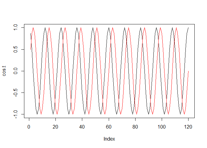
A discrete Fourier serie is an elegant way to model such cyclical trends. We will then create two waves, based on cosinus and sinus function.
To do this, we need to define the period of the cycle, that is the number of time after which we expect the system to return to a similar state. Because we have monthly data, we consider period = 12, because the value at a given month should be close to the value 12 month before. For a diurnal cycle, the period could well be 24h.
period <- 12
cos.t <- cos(2 * pi * seq(12*10)/period) # Out data set is 10 years*12 month large
sin.t <- sin(2 * pi * seq(12*10)/period)
c.Four <- rbind(cos.t, sin.t)

plot(cos.t, type = "l")
lines(sin.t, type = "l", col = "red")
 To fit a seasonal model,
- we estimate B, the auto-regressive parameter
- we estimate u, the drift
- we estimate Q, the standard-deviation of the random-walk
- we estimate C, the covariate “slopes”
- Z = 1
- a = 0
- we estimate mu (initial latent-state)
- we estimate R (noise aroung the latent state)
mod.list.sais <- list(B = matrix("autoreg"), U = matrix("drift"), Q = matrix("sd_proc"),
                      c = c.Four, C = matrix(c("c.cos", "c.sin")),
                     Z = matrix(1), A = matrix(0), R = matrix("sd_obs"),
                     x0 = matrix("init.state"))
Let’s fit the model.
fit.sais <- MARSS(Datat["Unicells",], model = mod.list.sais,
                  method = "BFGS")
## Success! Converged in 71 iterations.
## Function MARSSkfas used for likelihood calculation.
##
## MARSS fit is
## Estimation method: BFGS
## Estimation converged in 71 iterations.
## Log-likelihood: -133.4814
## AIC: 280.9629   AICc: 281.9629
##
##               Estimate
## R.sd_obs        0.0643
## B.autoreg       0.6774
## U.drift        -0.0522
## Q.sd_proc       0.4517
## x0.init.state   1.1645
## C.c.cos        -0.1635
## C.c.sin         0.1302
## Initial states (x0) defined at t=0
##
## Standard errors have not been calculated.
## Use MARSSparamCIs to compute CIs and bias estimates.
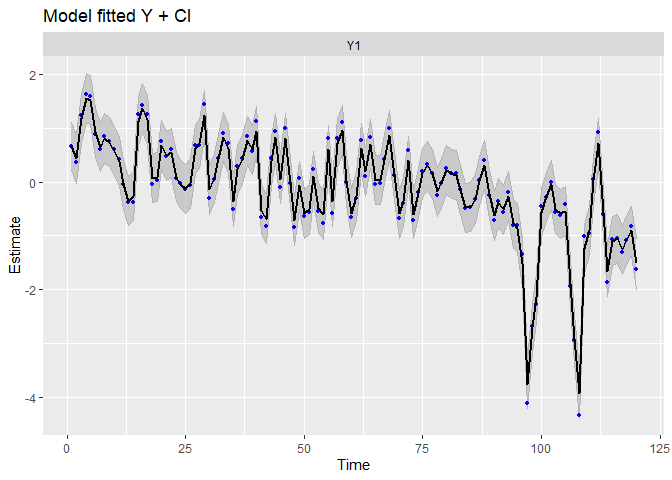
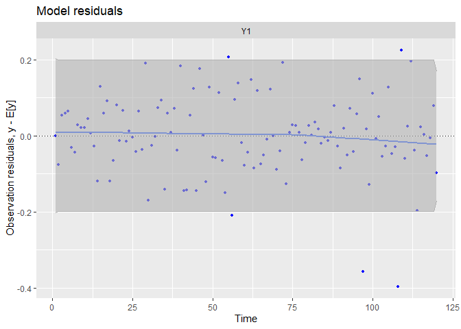
And evaluate it.
autoplot(fit.sais, plot.type = c("model.ytT", "model.resids", "qqplot.model.resids", "acf.model.resids"))
## plot.type = model.ytT
## Hit <Return> to see next plot (q to exit):
## plot.type = model.resids
## Hit <Return> to see next plot (q to exit):
## plot.type = qqplot.model.resids
## Hit <Return> to see next plot (q to exit):
## plot.type = acf.model.resids
## Finished plots.
The fit and the residual plots are still pretty good. The line of the latent states my be a little less close to the observed data, which is a good thing : over-fitting (reproducing strictly the data by capturing irrelevant noise) is a problem when we want to make good prediction!
Let’s forecast! The code is a little bit more complicated here, because we have to furnish new value of the covariates.
fr.sais <- forecast.marssMLE(fit.sais, h = 24, newdata = list(c = rbind(
  cos.t = cos(2 * pi * seq(24)/12),
  sin.t = sin(2 * pi * seq(24)/12)
    )))

autoplot(fr.sais)
The predictions are similar to the ones from the auto-regressive model (the system should return to its mean state), but we now expect seasonal variation.
Quantification of predictive accuracy
One efficient way to evaluate the predictive accuracy of a model is to confront its prediction to a “test” data set (as opposed to a training set). Remember we stopped the time-series at the end of 1989. We can now use the two following years, 1990 and 1991, to estimate the accuracy of our models.
yr_frst <- 1990
yr_last <- 1991
# Filtrer entre yr_frst et yr_last
PlankTest <- D[D[, "Year"] >= yr_frst & D[,
    "Year"] <= yr_last, ]

DataTest <- ts(PlankTest[, c("Year", "Month", "Temp", "TP", "pH", "Unicells")],
               frequency = 12, start = c(Plank[1, "Year"], Plank[1, "Month"]))
We can easily represent the prediction and the the observed data points using the following code. Did the system returned to its average state in 1990?
plot(fr.sais)
points(121:144, DataTest[, "Unicells"], pch = 16, col = "red")
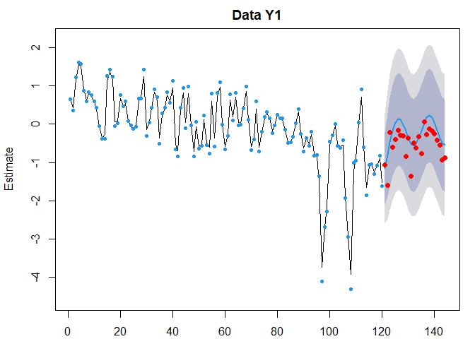
Wahou, that is not bad! The decreasing trend was indeed not to continue. It seems the seasonnal variation is now a little bit greater than it was, on average.
We can now quantify the futur predictive accuracy of the model using the Root-Mean-Square error around the observed values of the test data set. Note that the accuracy function provides many other measures of accuracy.
RMSE is on the scale of the response data (g, cm…). In our case, interpreting the RMSE is hard because our data is on the standard-deviation scale. It will always be up to you, as biologists or ecologists, to decide if the RMSE is sufficiently low to consider the prediction sufficiently effective in your system. And it depends on each system! A 10 g RMSE is almost a perfect fit if you want to predict the weight of an elephant, but may be a disaster if you want to predict zooplankton biomass per cube meters.
# Intercept
accuracy(fr.int, x = DataTest[,"Unicells"])[,"RMSE"]
## Training set           Y1     Test set
##    0.9892070    0.9892070    0.5794352
# Drift
accuracy(fr.drift, x = DataTest[,"Unicells"])[,"RMSE"]
## Training set           Y1     Test set
##    0.7807368    0.7807368    0.9456530
# Random walk
accuracy(fr.randrift, x = DataTest[,"Unicells"])[,"RMSE"]
## Training set           Y1     Test set
##    0.8007194    0.8007194    1.1162089
# Auto-regression
accuracy(fr.auto, x = DataTest[,"Unicells"])[,"RMSE"]
## Training set           Y1     Test set
##    0.7522220    0.7522220    0.4453414
# Saisonalité
accuracy(fr.sais, x = DataTest[,"Unicells"])[,"RMSE"]
## Training set           Y1     Test set
##    0.7361016    0.7361016    0.3986146
The final, most complex model including seasonality seems to reproduces better both the training set (1980-1989) and the test set (1990-1991). It is only slightly better than the auto-regressive model without seasonality. Note that the drift and random-walk+drift model have quite low RMSE on the training set, but produced far worst out-of-sample predictions!
Conclusion
Time-series modeling is a complex and specific task, which is grounded on concepts which are generally absent from our general statistical background. System dynamic may at first be counter-intuitive, as in the above example, when the tendency (a concept we are strongly attached to, because of linear regression) failed to accurately capture the future dynamic of the system. At the same time, it showed you the need to analyze dynamic systems with adapted tools.
We hope this gentle tutorial gave you a good introduction at this new task. Good success!!