Classe de maître avec Guillaume Blanchet

Avril 2022

Ouvrir les données
Question 1 - Relation esp - env
Relation espace - env pour la communauté
- Moran’s eigenvector maps pour variables spatiales

Ce code permet de reproduire l’analyse de données improvisée par Guillaume Blanchet lors de sa participation à l’activité Classe de Maître du Numérilab.

Cet atelier vous est offert à titre de divertissement, mais il ne devrait en aucun cas servir de référence pour la mise en place de solutions d’analyse de données dans le cadre d’un vrai projet.

Bonne lecture!

Ouvrir les données

sp <- readRDS("sp2015.RDS")
env <- readRDS("env2015.RDS")

library(mapview)

## Warning: le package 'mapview' a été compilé avec la version R 4.1.3

mapview(sp)

# mapview(env) # Même que sp (on vient de le regarder !)

head(env)

## Simple feature collection with 6 features and 8 fields
## Geometry type: POINT
## Dimension:     XY
## Bounding box:  xmin: 1115906 ymin: 447007 xmax: 1255002 ymax: 500183
## Projected CRS: NAD83 / MTQ Lambert
##      surface.temperature bottom.temperature bottom.salinity      seal ice
## 5947                17.8                5.1            29.9 67.774815 126
## 5948                15.7                0.9            32.1 13.516211 126
## 5949                15.8                0.9            31.8 26.233578 126
## 5950                15.2                1.0            32.3  2.117578 122
## 5951                15.2                0.9            32.2  5.334104 122
## 5952                13.9                1.3            32.7  3.299375 122
##          slope coarsness surfaceBottomTempDiff                 geometry
## 5947 0.1209286 0.6952367                  12.7   POINT (1115906 447007)
## 5948 0.1679912 2.4392456                  14.8 POINT (1186868 469659.8)
## 5949 0.2088341 3.0286032                  14.9 POINT (1201008 469630.5)
## 5950 0.1394752 0.1658933                  14.2 POINT (1209888 492226.4)
## 5951 0.3368716 6.1529986                  14.3 POINT (1231779 491539.2)
## 5952 0.2605593 5.3716641                  12.6   POINT (1255002 500183)

Question 1 - Relation esp - env

library(sf)

## Linking to GEOS 3.9.1, GDAL 3.2.1, PROJ 7.2.1

library(vegan)

## Warning: le package 'vegan' a été compilé avec la version R 4.1.2

## Le chargement a nécessité le package : permute

## Warning: le package 'permute' a été compilé avec la version R 4.1.2

## Le chargement a nécessité le package : lattice

## This is vegan 2.5-7

# Retirer géométrie
spDat <- st_drop_geometry(sp)
envDat <- st_drop_geometry(env)

# Ordination canonique
spHell <- decostand(spDat, method = "hellinger")

RDA <- rda(spHell, scale(envDat))
# summary(RDA)

# Graph brute !
plot(RDA, scaling = 2) # Relation entre les flèches

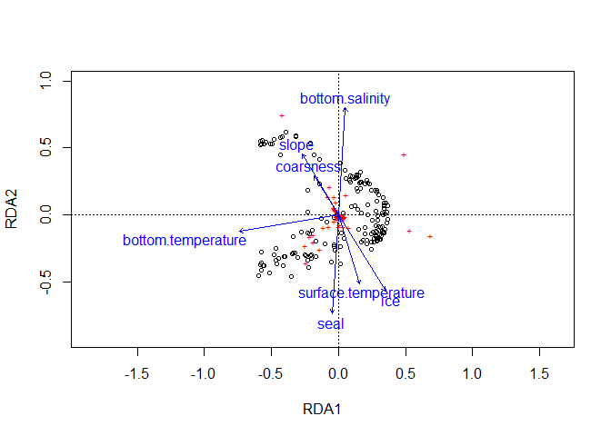
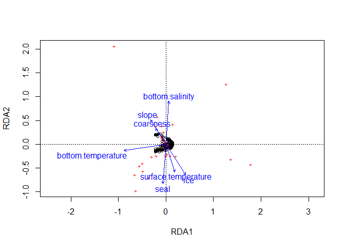
plot(RDA, scaling = 1) # Relation entre les sites

#---------------------
# Graph un peu mieux !
#---------------------
# Importance Axes
poidsAxe <- eigenvals(RDA)/ sum(eigenvals(RDA))

# position espèces dans le biplot
spAxe <- scores(RDA,
                choices = 1:2,
                display = "species",
                scaling = 2)

# position variables environmentale dans le biplot
envAxe <- scores(RDA,
                 choices = 1:2,
                 display = "bp",
                 scaling = 2)

# position sites dans le biplot
siteAxe <- scores(RDA,
                  choices = 1:2,
                  display = "sites",
                  scaling = 2)
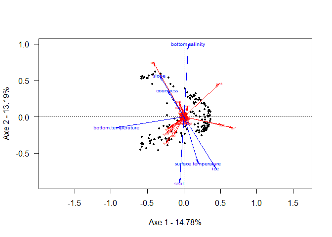
# Base du graph
plot(RDA,
     xlab = paste0("Axe 1 - ",round(poidsAxe[1],4) * 100,"%"),
     ylab = paste0("Axe 2 - ",round(poidsAxe[2],4) * 100,"%"),
     type = "n",
     las = 1,
     scaling = 2)

# site
points(siteAxe, pch = 19, cex = 0.5)

# sp
arrows(x0 = 0,
       y0 = 0,
       x1 = spAxe[,1],
       y1 = spAxe[,2],
       angle = 10,
       length = 0.1,
       col = "red")

text(spAxe,
     labels = rownames(spAxe),
     col = "red",
     cex = 0.4)

# env
arrows(x0 = 0,
       y0 = 0,
       x1 = envAxe[,1],
       y1 = envAxe[,2],
       angle = 10,
       length = 0.1,
       col = "blue")

text(envAxe,
     labels = rownames(envAxe),
     col = "blue",
     cex = 0.6)

Relation espace - env pour la communauté

Moran’s eigenvector maps pour variables spatiales

library(adespatial)

## Warning: le package 'adespatial' a été compilé avec la version R 4.1.3

## Registered S3 methods overwritten by 'adegraphics':
##   method         from
##   biplot.dudi    ade4
##   kplot.foucart  ade4
##   kplot.mcoa     ade4
##   kplot.mfa      ade4
##   kplot.pta      ade4
##   kplot.sepan    ade4
##   kplot.statis   ade4
##   scatter.coa    ade4
##   scatter.dudi   ade4
##   scatter.nipals ade4
##   scatter.pco    ade4
##   score.acm      ade4
##   score.mix      ade4
##   score.pca      ade4
##   screeplot.dudi ade4

## Registered S3 method overwritten by 'spdep':
##   method   from
##   plot.mst ape

## Registered S3 methods overwritten by 'adespatial':
##   method             from       
##   plot.multispati    adegraphics
##   print.multispati   ade4       
##   summary.multispati ade4

#?mem #Pour les MEMs super spécifique

# pcnm - Général mais pas optimal (bon pour l'illustration)
PCNM <- pcnm(dist(st_coordinates(sp))) # dans vegan

# calcul R2a
vp <- varpart(spHell,
               PCNM$vectors,
               PCNM$vectors)

## Warning: collinearity detected in cbind(X1,X2): mm = 184, m = 92

# Forward selection sur les variables spatiales (PCNM)
fs <- forward.sel(Y = spHell,
                  X = PCNM$vectors,
                  adjR2thresh = vp$part$fract[1,3],
                  alpha = 0.06) # dans adespatial

## Testing variable 1
## Testing variable 2
## Testing variable 3
## Testing variable 4
## Testing variable 5
## Testing variable 6
## Testing variable 7
## Testing variable 8
## Testing variable 9
## Testing variable 10
## Testing variable 11
## Testing variable 12
## Testing variable 13
## Testing variable 14
## Testing variable 15
## Testing variable 16
## Testing variable 17
## Testing variable 18
## Testing variable 19
## Testing variable 20
## Testing variable 21
## Testing variable 22
## Testing variable 23
## Testing variable 24
## Testing variable 25
## Testing variable 26
## Testing variable 27
## Testing variable 28
## Testing variable 29
## Testing variable 30
## Testing variable 31
## Testing variable 32
## Procedure stopped (alpha criteria): pvalue for variable 32 is 0.075000 (> 0.060000)

fs

##    variables order          R2      R2Cum   AdjR2Cum        F pvalue
## 1      PCNM5     5 0.045437491 0.04543749 0.03943395 7.568453  0.001
## 2      PCNM2     2 0.039319304 0.08475679 0.07317144 6.787759  0.001
## 3      PCNM7     7 0.028906271 0.11366307 0.09672669 5.120270  0.001
## 4     PCNM13    13 0.026701675 0.14036474 0.11832281 4.845615  0.001
## 5      PCNM8     8 0.024751000 0.16511574 0.13818399 4.595134  0.001
## 6      PCNM3     3 0.021682337 0.18679808 0.15511489 4.106089  0.001
## 7     PCNM19    19 0.016983719 0.20378180 0.16735351 3.263564  0.005
## 8      PCNM6     6 0.016047654 0.21982945 0.17876784 3.126552  0.002
## 9     PCNM36    36 0.015528774 0.23535823 0.18978355 3.066593  0.001
## 10    PCNM20    20 0.014508823 0.24986705 0.19985818 2.901250  0.005
## 11    PCNM11    11 0.013786430 0.26365348 0.20929233 2.789689  0.004
## 12     PCNM1     1 0.013695869 0.27734935 0.21875605 2.804936  0.007
## 13     PCNM4     4 0.013591923 0.29094127 0.22823540 2.817838  0.009
## 14    PCNM92    92 0.013477706 0.30441898 0.23771943 2.828923  0.004
## 15    PCNM10    10 0.013461742 0.31788072 0.24731666 2.861600  0.002
## 16    PCNM21    21 0.013102116 0.33098283 0.25664759 2.820114  0.009
## 17    PCNM24    24 0.012770203 0.34375304 0.26573766 2.782701  0.004
## 18    PCNM15    15 0.012705285 0.35645832 0.27488262 2.803471  0.005
## 19    PCNM17    17 0.011332287 0.36779061 0.28259927 2.527410  0.006
## 20    PCNM33    33 0.010810143 0.37860075 0.28982943 2.435503  0.014
## 21     PCNM9     9 0.010452063 0.38905282 0.29675144 2.378007  0.022
## 22    PCNM23    23 0.010250380 0.39930320 0.30353994 2.354853  0.015
## 23    PCNM12    12 0.010102585 0.40940578 0.31025493 2.343494  0.014
## 24    PCNM16    16 0.009679705 0.41908549 0.31657116 2.266151  0.017
## 25    PCNM18    18 0.009384354 0.42846984 0.32263092 2.216660  0.028
## 26    PCNM14    14 0.008966696 0.43743654 0.32828243 2.135825  0.023
## 27    PCNM30    30 0.008964658 0.44640119 0.33401647 2.153725  0.028
## 28    PCNM75    75 0.008769852 0.45517105 0.33960127 2.124741  0.034
## 29    PCNM26    26 0.008554484 0.46372553 0.34500828 2.089671  0.029
## 30    PCNM28    28 0.007724472 0.47145000 0.34947693 1.899880  0.047
## 31    PCNM72    72 0.007523453 0.47897346 0.35376553 1.862718  0.050

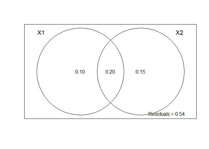
# Partition de la variation
vpRes <- varpart(spHell,
                 scale(envDat),
                 PCNM$vectors[,fs$order])

## Warning: collinearity detected in X1: mm = 8, m = 7

## Warning: collinearity detected in cbind(X1,X2): mm = 39, m = 38

vpRes

##
## Partition of variance in RDA
##
## Call: varpart(Y = spHell, X = scale(envDat), PCNM$vectors[, fs$order])
##
## Explanatory tables:
## X1:  scale(envDat)
## X2:  PCNM$vectors[, fs$order]
##
## No. of explanatory tables: 2
## Total variation (SS): 100.64
##             Variance: 0.629
## No. of observations: 161
##
## Partition table:
##                      Df R.squared Adj.R.squared Testable
## [a+b] = X1            7   0.33639       0.30603     TRUE
## [b+c] = X2           31   0.47897       0.35377     TRUE
## [a+b+c] = X1+X2      38   0.58501       0.45575     TRUE
## Individual fractions                                    
## [a] = X1|X2           7                 0.10199     TRUE
## [b]                   0                 0.20404    FALSE
## [c] = X2|X1          31                 0.14972     TRUE
## [d] = Residuals                         0.54425    FALSE
## ---
## Use function 'rda' to test significance of fractions of interest

plot(vpRes)